Recently I set out to hold a
Battleship programming
tournament here among some of the undergraduates. Naturally, I myself
wanted to win. So, I got to thinking about the game, and developed what
I like to call "the linear theory of battleship". A demonstration of the
fruits of my efforts can be found
here. Below, my
aim is to guide you through how I developed this theory, as an exercise
in using physics to solve an interesting unknown problem. This is one of
the things I really love about physics, the fact that obtaining an
education in physics is essentially an education in reasoning and
thinking through complicated problems, along with an honestly short list
of tips and tricks that have proven successful for tackling a wide range
of problems. So, how do we develop the linear theory of battleship?
First we need to quantify what we know, and what we want to know.
The Goal
So, how does one win Battleship? Since the game is about sinking your
opponents ships before they can sink yours, it would seem that a good
strategy would be to try to maximize your probability of getting a hit
every turn. Or, if we knew the probabilities of there being a hit on
every square, we could guess each square with that probability, to keep
things a little random. So, let's try to represent what we are after. We
are after a whole set of numbers $$ P_{i,\alpha} $$ where i ranges
from 0 to 99 and denotes a particular square on the board, and alpha can
take the values C,B,S,D,P for carrier, battleship, submarine, destroyer,
and patrol boat respectively. This matrix should tell us the probability
of there being the given ship on the given square. E.g. $$ P_{53,B} $$
would be the probability of there being a battleship on the 53rd square.
If we had such a matrix, we could figure out the probability of there
being at hit on every square by summing over all of the ships we have
left, i.e. $$ P_i = \sum_{\text{ships left}} P_{i, \alpha } $$
The Background
Alright, we seem to have a goal in mind, now we need to quantify what we
have to work with. Minimally, we should try to measure the probabilities
for the ships to be on each square given a random board configuration.
Let's codify that information in another matrix $$ B_{i,\alpha} $$
where B stands for 'background', i runs from 0 to 99, and alpha is
either C,B,S,D, or P again, and stands for a ship. This matrix should
tell us the probability of a particular ship being on a particular spot
on the board assuming our opponent generated a completely random board.
This is something we can measure. In fact, I wrote a little code to
generate random Battleship boards, and counted where each of the ships
appeared. I did this billions of times to get good statistics, and what
I ended up with is a little interesting. You can see the results for
yourself over at my results exploration
page by changing
the radio buttons for the ship you are interested in, but I have some
screen caps below. Click on any of them to embiggen.
All
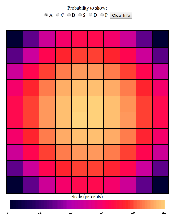
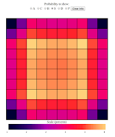
First of all, lets look at the sum of all of the ship probabilities, so
that we have the probability of getting a hit on any square for any ship
given a random board configuration, or in our new parlance $$ B_i =
\sum_{\alpha={C,B,S,D,P} } B_{i,\alpha} $$ The results:
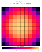
shouldn't be too surprising. Notice first that we can see that my
statistics are fairly good, because our probabilities look more or less
smooth, as they ought to be, and show nice left/right up/down symmetry,
which it ought to have. But as you'll notice, on the whole there is
greater probability to get a hit near the center of the board than near
the edges, an especially low probability of getting a hit in the
corners. Why is that? Well, there are a lot more ways to lay down a ship
such that there is a hit in a center square than there are ways to lay a
ship so that it gives a hit in a corner. In fact, for a particular ship
there are only two ways to lay it so that it registers a hit in the
corner. But, for a particular square in the center, for the Carrier for
example there are 5 different ways to lay it horizontally to register a
hit, and 5 ways to lay it vertically, or 10 ways total. Neat. We see
entropy in action.
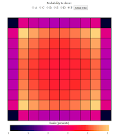
Carrier
Next let's look just at the Carrier:
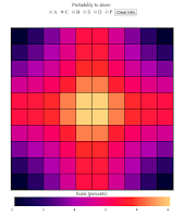
Woah. This time the center is very heavily favored versus the edges.
This reflects the fact that the Carrier is a large ship, occupying 5
spaces, basically no matter how you lay it, it is going to have a part
that lies near the center.
Battleship
Now for the Battleship:
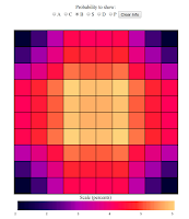
This is interesting. This time, the most probable squares are not the
center ones, but the not quite center ones. Why is that? Well, we saw
that for the Carrier, the probability of finding it in the center was
very large, and so respectfully, our battleship cannot be in the center
as often, as a lot of the time it would collide with the Carrier. Now,
this is not because I lay down the Carrier first, my board generation
algorithm assigns all of the boards at once, and just weeds out invalid
ones, this is a real entropic effect. So here we begin to see some
interesting Ship-Ship interactions in our probability distributions. But
notice again that on the whole, the battleship should also be found near
the center as it is also a large ship.
Sub / Destroyer
Next let's look at the sub / destroyer. First thing to note is that our
plot should be the same for both of these ships as they are both the
same length.
Here we see an even more pronounced effect near the center. The Subs and
Destroyers are 'pushed' out of the center because the Carriers and
Battleships like to be there. This is a sort of entropic repulsion.
Patrol Boat
Finally, let's look at the patrol boat:
The patrol boat is a tiny ship. At only two squares long, it can fit in
just about anywhere, and so we see it being strongly affected by the
affection the other ships have for the center. Neat stuff. So, we've
experimentally measured where we are likely to find all of the
battleship ships if we have a completely random board configuration.
Already we could use this to make our game play a little more effective,
but I think we can do better.
The Info
In fact, as a game of battleship unfolds, we learn a good deal of
information about the board. In fact on every turn we get a great deal
of information about a particular spot on the board, our guess. Can we
incorporate this information into our theory of battleship? Of course we
can, but first we need to come up with a good way to represent this
information. I suggest we invent another matrix! Let's call this one $$
I_{j,\beta} $$ Where I is for 'information', j goes from 0 to 99 and
beta marks the kind of information we have about a square, let's let it
take the values M,H,C,B,S,D,P, where M means a miss, H means a hit, but
we don't know which ship, and CBSDP mark a particular ship hit, which we
would know once we sink a ship. This matrix will be a binary one, where
for any particular value of j, the elements will all be 0 or 1, with
only one 1 sitting at the spot marking our information about the square,
if we have any. That was confusing. What do I mean? Well, let's say its
the start of the game and we don't know a darn thing about spot 34 on
the board, then I would set $$
I_{34,M}=I_{34,H}=I_{34,C}=I_{34,B}=I_{34,S}=I_{34,D}=I_{34,P}=0
$$ that is, all of the columns are zero because we don't have any
information. Now let's say we guess spot 34 and are told we missed, now
that row of our matrix would be $$ I_{34,M} = 1 \quad
I_{34,H}=I_{34,C}=I_{34,B}=I_{34,S}=I_{34,D}=I_{34,P}=0 $$ so that
we put a 1 in the column we know is right, instead, if we were told it
was a hit, but don't know which ship it was: $$ I_{34,H} = 1 \quad
I_{34,M}=I_{34,C}=I_{34,B}=I_{34,S}=I_{34,D}=I_{34,P}=0 $$ and
finally, lets say a few turns later we sink our opponents sub, and we
know that spot 34 was one of the spots the sub occupied, we would set:
$$ I_{34,S} = 1 \quad
I_{34,M}=I_{34,H}=I_{34,C}=I_{34,B}=I_{34,D}=I_{34,P}=0 $$ This
may seem like a silly way to codify the information, but I promise it
will pay off. As far as my Battleship Data
Explorer goes,
you don't have to worry about all this nonsense, instead you can just
click on squares to set their information content. Note: shift-clicking
will let you cycle through the particular ships, if you just regular
click it will let you shuffle between no information, hit, and miss.
The Theory
Alright if we decide to go with my silly way of codifying the
information, at this point we have two pieces of data, $$ B_{i,\alpha}
$$ our background probability matrix, and $$ I_{j,\beta} $$ our
information matrix, where what we want is $$ P_{i,\alpha} $$ the
probability matrix. Here is where the linear part comes in. Why don't we
adopt the time honored tradition in science of saying that the
relationship between all of these things is just a linear one? In matrix
language that means we will choose our theory to be $$ P_{i,\alpha} =
B_{i,\alpha} + \sum_{j=[0,..,99],\beta={M,H,C,B,S,D,P}}
W_{i,\alpha,j,\beta} I_{j,\beta} $$ Whoa! What the heck is that!?
Well, that is my linear theory of battleship. What the equation is
trying to say is that I will try to predict the probability of a
particular ship being in a particular square by (1) noting the
background probability of that being true, and (2) adding up all of the
information I have, weighting it by the appropriate factor. So here, P
is our probability matrix, B is our background info matrix, I is our
information matrix, and W is our weight matrix, which is supposed to
apply the appropriate weights. That W guy seems like quite the monster.
It has four indexes! It does, so let's try to walk through what they all
mean. Here: $$ W_{i,\alpha,j,\beta} $$ is supposed to tell us: "the
extra probability of there being ship alpha at location i, given the
fact that we have the situation beta going on at location j" Read that
sentence a few times. I'm sorry its confusing, but it is the best way I
could come up with explaining W in english. Perhaps a visual would help.
Behold the following: (click to embiggen)
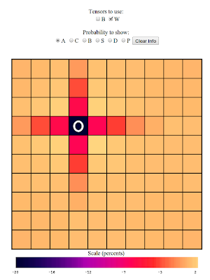
That is a picture of $$ W_{i,C,33,M} $$ that is, that is a picture of
the extra probabilities for each square (i is all of them), of there
being a carrier, (alpha=C) given that we got a miss (beta=M) on square
33, (j=33). You'll notice that the fact that we saw a miss affects some
of the squares nearby. In fact, knowing that there was a miss on square
33 means that the probability that the carrier will be found on the
adjacent squares is a little lower (notice on the scale that the nearby
values are negative), because there are now fewer ways the carrier could
be on those squares without it overlapping over into square 33. Let's
try another:
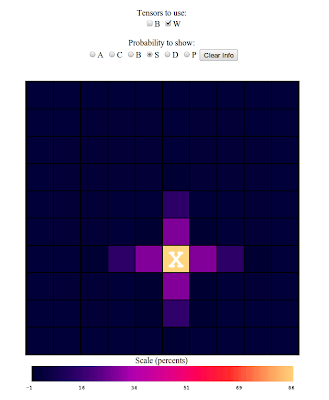
That is a picture of $$ W_{i,S,65,H} $$ that is, it's showing the extra
probability of there being a submarine (alpha=S), at each square (i is
all of them, since its a picture with 100 squares), given that we
registered a hit (beta=H) on square 65 (j=65). Here you'll notice that
since we marked a hit on square 65, it is very likely that we will also
get hits on the squares just next to this one, as we could have
suspected. In the end, by assuming our theory has this linear form, the
benefit we gain is that by doing the same sort of simulations I did to
generate the background information, I can back out what the proper
values should be for this W matrix. By doing billions and billions of
simulations, I can ask, for any particular set of information, I, what
the probabilities are P, and solve for W. Given that the problem is
linear, this solving step is particularly easy for me to do.
The Results
In the end, this is exactly what I did. I had my computer create
billions of different battleship boards, and figure out what the proper
values of B and W should be for every square of the matrix. I put all of
those results together in a way that I hope is easy to explore up at the
Fancy Battleship Results
Page, where you
are free to explore all of the results yourself. In fact, the way it's
set up, you can even use the Superduper Results
Page as a sort of
Battleship Cheat Sheet. Have it open while you play a game of
battleship, and it will show you the probabilities associated with all
of the squares, helping you make your next guess. I've used the page
while playing a few games of battleship online, and have had some
success, winning 9 of the 10 games I played against the computer player.
Of course, this linear theory isn't everything...
Why Linear isn't everything
But at the end of the day, we've made a pretty glaring assumption about
the game of battleship, namely that all of the information on the board
adds in a linear way. Another way to say that is that in our theory of
battleship, we have a principle of superposition. Another way to say
that is that in this theory, what you think is happening in a particular
square is just the sum of the results from all of the squares,
independent of one another. Another way to say that is to show it with
another picture. Consider the following:
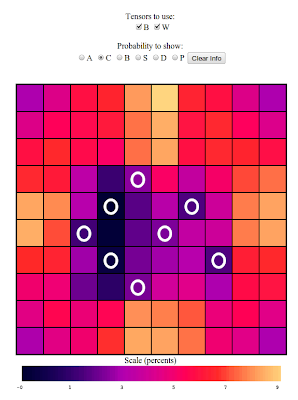
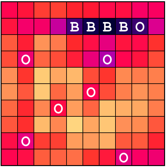
Here, I've specified a bunch of misses, and am asking for the
probability of there being a Carrier on all of the positions of the
board. If you look in the center of that cluster of misses, especially
in the inner left of the bunch, you'll see that the linear theory tells
me that there is a small but finite chance that the Carrier is located
on those squares. But if you stop to look at the board a little bit,
you'll notice that I've arranged the misses such that there is a large
swatch of squares in the center of the cluster where the Carrier is
strictly forbidden. There is no way it can fit such that it touches a
lot of those central squares. This is an example of the failure of the
linear model. All the linear model knows is that in the spots nearby
misses there is a lower probability of the ship being there, but what it
doesn't know to do is look at the arrangement of misses and check to see
whether there is any possible way the ship can fit. This is a nonlinear
effect, involving information at more than one square at a time. It is
these kinds of effects that this theory will miss, but as you'll notice,
it still does pretty well. Even though it reports a finite positive
probability of the Carrier being inside the cluster, the value it
reports is a very small one, about 1 percent at most. So the linear
theory will have corrections at the 1 percent level or so, but that's
pretty good if you ask me.
Summary
And so it is. I've tried to develop a linear theory for the game
Battleship, and display the results in a Handy Dandy Data
Explorer. I
encourage you to play around with the website, use it to win games of
Battleship, and in the comments, point out interesting effects, things
you think I've missed, or ideas for how to come up with linear theories
of other things.
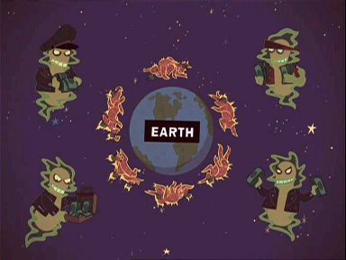
 Marty McFly realizes he is running out of time to submit his solution