Consider the site reborn. After nearly a decade hiatus, let's see if we can
get this old engine purring again. This time the site is being built statically
with Nikola, exists as a github
repo and is being served on github
pages. Still need to edit some of the old posts
for correctness and need to develop the theme more, but consider this a
new beginning.
I loved this video because I've had a number of experiences like this. My
favorite reaction that I've ever gotten happened in 2007. I was on a trip
during college with other college kids, and I was placed in a hotel room with
some guys who went to another school. We met for the first time while
unpacking, and naturally we asked each other what we were studying. Turns out
my new roommate was majoring in international business, something I knew
nothing about. Not wanting to alienate a total stranger I was going to be
sleeping in the same room with, I asked him questions and told him that his
chosen major sounded interesting and important. I told him that I studied
physics, and when he asked me what that meant I told him how I had worked on
modeling cell division. My new
roommate responded, "You must have a special kind of brain for that."
This anecdote has stuck with me for a couple of reasons-- first because
"special kind of brain" is a funny turn of phrase, and second because I think
it's a perfect example of how an attempt at a flattering response can actually
create some uncomfortable social distance between people.
"Special kind of brain" was my roommate's way of expressing how intelligent he
thought I was. (Or, as Zach put it in Katie's video, "You must be soooooo
smart!") His reaction hinged upon the assumption that what I was interested in
doing was so far beyond the understanding of ordinary folk that I could be set
apart as a member of an elite group. Instead of being merely complimentary,
his comment held me at arms' length. His reaction wasn't something I took
offense to, but it made me uncomfortable to hear that he considered me an
outsider of sorts based on my professed interests.
Speaking more generally, the notion that scientific professionals are set apart
from other people as members of a professional group isn't so ridiculous. After
all, these days people's lives are often defined by their careers. (And of
course scientists aren't the only profession with associated negative
stereotypes-- Anyone know any good lawyer jokes?). But to me, thinking of
scientists as some kind of inscrutable cabal of geniuses is an exaggeration.
The truth is, not every scientist is a rocket-powered superbrain. Quite the
opposite-- scientists make silly mistakes all the time. Being a scientist is
a technical profession requiring years of training like law, medicine, or
accounting: there are a few practitioners who really are exceptionally smart,
while most of the others aren't.
The even more disappointing truth is that being a scientist is actually usually
pretty mundane. Don't get me wrong-- the long-term goals of making new
discoveries and developing new insights into the world around us are exactly
why I like my job. I just mean that the day-to-day labor involved can be as
tedious as any other profession. I sit in my cubicle and code (debug)
endlessly on my laptop, or I read books and research papers to learn new things
about my field. Most days don't get much more action-packed than that. In a
lot of ways it's like any other office job. Aside from the end goal of
research, working as a scientist is not so special.
Another reaction that I get when I say I study physics is one of apprehensive
disappointment. (Zach's pronunciation of 'ohhhhhh...' combining equal parts
boredom and distaste was dead on.) I don't think I need to dwell on this too
long-- it is undeniably unpleasant for me when I hear this. Upon hearing that
I'm a scientist, otherwise polite, kind people will suddenly lose their cool
and be unable to hide the fact that my profession conjures up memories of
boredom and frustration. ("Oh, man. I HATED physics in high school.") As
Katie Mack puts it at the end, "polite interest is the way to go."
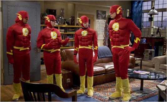
"Have you ever seen the Big Bang Theory? Is that what physicists are really like? I bet it is. I mean, no offense."
There's another type of off-putting reaction that comes up sometimes, which is
commenting (jokingly or not) that I'm similar to familiar caricature of
scientists that appear in popular culture. "You're just like Sheldon Cooper!"
is a comment I've heard more times than I care to say. I know that The Big Bang
Theory is a popular show, but frankly I dislike being associated I with
characters that are cartoonishly depicted as condescending and socially
tone-deaf [3]. Now, I appreciate that some
people, when meeting others for the first time, like to demonstrate familiarity
with others' jobs, but to me it just seems that making a pop culture references
to another person's profession is just a bad way to go. I find this to be a
safe bet when meeting anyone, not just scientists, simply because popular
culture isn't a great way to learn about anyone else's job. Try telling the
next lawyer you meet that they remind you of Saul
Goodman, and see how they react.
So, what is there for physicists (and other scientists) to do when this
happens? The most facile answer to this question is for us to grow a thicker
skin and suck it up. Just ignore it when people have disparaging reactions
upon first meeting us, and find a way to get past this in conversation. The
thing is, I personally am not good enough at hiding my own negative reaction
upon hearing these kinds of obnoxious remarks. Ideally, I'd like to make
conversation easier by finding a way to avoid them altogether.
I can't change the way other people react to learning about my profession, but
I can change how I present myself. Personally, I have given up on telling
people that I'm in the physics department. Instead, when asked "what do you
study in grad school?" I tell then exactly what I'm up to-- I study how
infectious diseases spread through human and animal communities. I've found
that I get a much more relaxed reaction when I do this. The same people who may
have uncomfortable reactions to physics have enough familiarity with the idea
of epidemics to be a little more comfortable. And besides, everyone has some
amount of morbid curiosity about the next big plague that's going to kill us
all. (I realize that this may not be a viable strategy for some of my
colleagues who study nanoscience, magnetic materials, high-energy particles, or
other mainstream physics topics. I'm interested to hear if anyone else who
works in the sciences has come up with a different technique for breaking
through the "I'm a physicist" ice.)
A friend of mine once chastised me for doing this. "Why should you have to hide
what you're interested in?" he asked. "If they react badly to your profession,
is it really worth getting to know them?" To that I say that I'm still telling
them honestly what I'm interested in, I just sidestep the potentially negative
associations carried by the word "physics." And besides, just because someone
has a bad or obnoxious reaction to finding out that I'm a physicist doesn't
mean they aren't worth meeting. The fact remains that I've found this to be a
great way to keep the getting-to-know-you conversation light when meeting new
people for the first time. I wish I could wave a magic wand and make it so that
everyone was comfortable wih the idea of interacting with professional
scientists, but I can't. While I'm waiting for Bill
Nye
and Neil DeGrasse Tyson and others to humanize
the profession for the public, this is how I'll be introducing myself.
Katie Mack and Zach's video really got me thinking about how to talk to other
people about their jobs with more empathy-- avoiding flattery and
stereotyping, and doing my best to hide any negative visceral reactions evoked
by the thought of others' jobs and interests. One question that has occurred
to me is whether there are people in completely different professions
experience similarly frustrating reactions when they say what their jobs are.
Programmers, actuaries, office administrators, copy editors, art dealers,
karate instructors, gravediggers, lion-tamers, etc.: whoever you are, I want
to hear about any difficulties you may have had with telling other people what
you do in the comments below.
^
Image from New X-Men #121, written by Grant Morrison with art by Frank Quitely.
You can see some more of this particularly trippy story
here.
^
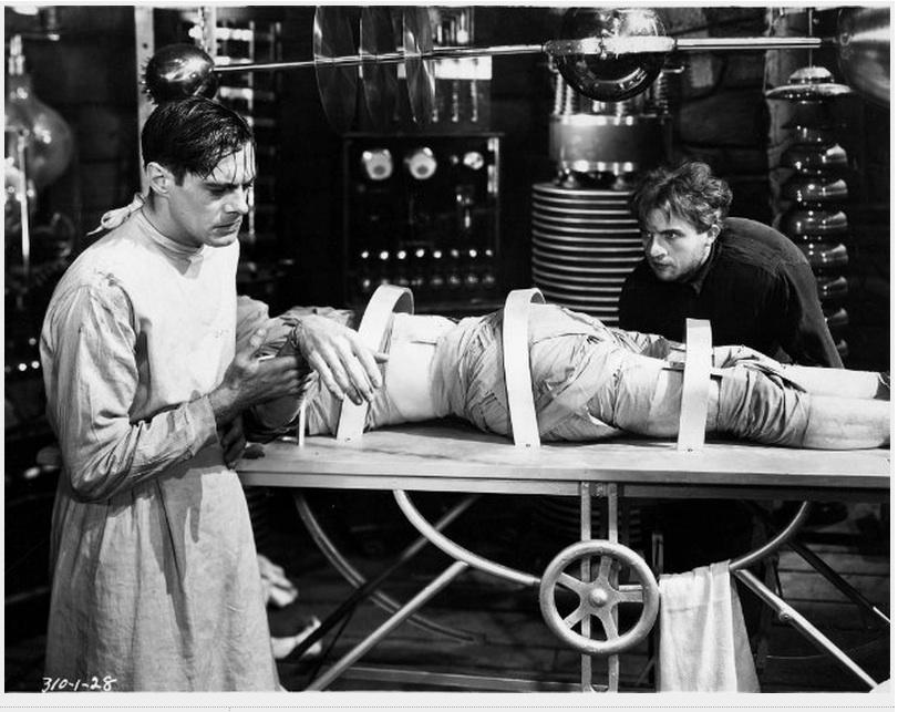
All of the imagery of Frankenstein's monster being brought to life with electricity
comes from James Whale's Frankenstein from 1931. Mary Shelley's original book contained no mention of
electricity, and instead remained eerily vague about the mechanisms for creating life.
^
Here is a really level-headed critique of The Big Bang Theory that I like a
lot. There isn't a ton of hand-wringing, and the author does talk about what the
show might consider doing differently. It was written three years ago.
A friend of mine (I’ll call him Ron), who knows that I study physics,
likes to talk to me about quantum mechanics. He’s an easy-going guy
and likes to joke around. “Hey, is it a particle or is it a wave today?”
he’ll say, or, “How many dimensions do we have now?” When the conversation
turns more serious, he tells me how he believes
in the “quantum universe,” which is greater than what we humans are
able to ordinarily perceive. He talks about consciousness, immortality,
spirits, and the great cosmic grandeur of the universe, all of which he
ties together with the label of “quantum.”
These conversations are strange to me. Both of us are using the same two words:
quantum mechanics. When Ron thinks about quantum mechanics, he associates it
with nonphysical concepts, like spirits. Through my time spent studying physics,
I’ve come to understand quantum mechanics as a theory describing the behavior of
atoms and subatomic particles.
For example, one day our chatting turned to the topic of medicine and how the
human body heals itself. Ron told me that the biggest problem with modern
medicine is that doctors think of the body as a physical object only.
Healing, he said, was a “quantum” effect. I told him that I could make a
pretty strong physical argument for why that wasn’t the case. He responded
with this story: Once, when playing football, he severely injured his knee.
The injury was so bad that he couldn’t bend it or move it. He didn’t have
health insurance and didn’t have the cash on hand to pay for medical treatment.
One day, he prayed to the universe that he would get better and a “tornado of
light came down” and healed his leg. Since then, Ron says, he’s always believed
in and respected the quantum universe.
I can’t tell Ron that what he described in his story didn’t happen,
that his experience was wrong or incorrect in some way. I wasn’t there,
so I can’t comment on the accuracy of his narrative. And even the story
of how his body healed out of the blue isn’t problematic: as far as I can
tell, decades after the story took place, Ron is in good shape and his leg
is doing fine. What I found objectionable about the story was how, in the
end, Ron attributed his healing to the miraculous intervention of quantum mechanics.
Quantum mechanics, in all of its glorious strangeness, is only relevant on
inconceivably small scales and at very, very low temperatures. One of the
reasons it took humans so long to develop the theory of quantum mechanics is
that quantum effects don’t readily appear in everyday life. My colleagues
who work to observe quantum mechanics in their experiments use lasers to manipulate
atoms
(objects that are 1/10,000,000,000th of a meter in size and weigh around
1/10,000,000,000,000,000,000,000,000th of a kilogram) at temperatures less than
1 Kelvin (about -459 degrees Fahrenheit). At larger sizes and temperatures
quantum effects are negligible. The human body is more than a meter long,
usually weighs around 50-100 kilograms and, if healthy, maintains a toasty
98 degrees Fahrenheit. Quantum mechanics is important at the atomic level,
but on the scales at which people interact with the world it hardly shows up
at all. So, even if Ron's leg heals as he said it did, I wouldn't give credit to quantum mechanics.[2]
I have been studying physics for years and still quantum mechanics
remains utterly baffling to me. The fact that such an abstract theory can tell us so
much about the world feels a little bit like a miracle. Quantum mechanics carries
with it a number of counterintuitive ideas like the
uncertainty principle[3]
entanglement, or parallel universes.
These ideas are so abstracted from every day life that the subject begins to take
on a supernatural quality. Physics no longer seems like physics-
it starts to sound like mysticism.
So it makes sense that contemporary culture has seized upon quantum mechanics
as a possible explanation for inexplicable things. The theory has so many
surprising results that it seems natural to extend it to encompass other things
that confuse us, like questions of consciousness. Furthermore, “quantum mechanics”
is a term that carries with it the weight of scientific legitimacy. If Ron had
said that he had been healed through witchcraft, laying on of hands, or alchemy
he would have sounded ridiculous, but attributing his experience to quantum effects
allows the story to borrow from the credible reputation of fact-based 20th century
science. What my friend doesn’t realize is that terminology is not what makes
quantum theory powerful: the scientific methodology supporting quantum mechanics
is what matters.
It’s important to keep separate quantum mechanics the physical theory and
quantum mechanics as a mystical cosmic principle. Despite how confusing it
is, quantum mechanics is an empirically motivated and mature theory that gives
us a framework to understand physical phenomena like radiation and chemical
bonding. This is fundamentally different from applying quantum mechanical
concepts to the nature of reality or consciousness. To do so may be a fun
philosophical parlor game, but it is baseless speculation without any evidence
to motivate the connection between quantum mechanics and the supernatural
that it begins with. This confusion is not just restricted to scientific laymen: there are
trained researchers working at well-respected research institutions
who also make the same mistake
my friend Ron does.
At the end of the day, speculation that the soul, the afterlife, ESP,
or whatever else are quantum effects is unscientific, but at least it
isn’t dangerous or harmful in the same way as climate change denial or
refusing to vaccinate your children.
It’s closer to something like intelligent design, which is
fundamentally confused about what science is.
(We physicists are truly thankful that there is no noisy political movement
to teach Deepak Chopra
alongside physics in high school classrooms.) So I won’t object to my
friends’ stories of sudden, unexpected recoveries from illness, but
I will react skeptically when I hear that healing has anything to do with quantum mechanics.
^ Credit where credit is due: I took this from XKCD. This may be one of
my favorite comics Randall Munroe has ever done. That it came out while
I was thinking about this piece was a great coincidence. (A cosmic
coincidence explainable through quantum entanglement? Probably not.)
^ Quantum mechanics may be just as mundane as any other materialistic physical
theory, but that doesn’t make it any less amazing. My favorite example is
how quantum mechanics allows us to understand why the sun works.
^ In case you didn't take the time to click on the link: Seriously, do
yourself a favor and click on the link . It's an essay from The Stone that very elegantly describes
how the uncertainty principle is far less cosmically mind-blowing than you
may have come to believe. It does a beautiful job bringing us back down to
earth and carefully explaining the scope of the principle. I must give it credit
for having inspired this piece in no small way.
Recently I finished reading John Mearsheimer's excellent political science book
The Tragedy of Great Power Politics. In this book, Mearscheimer lays out his
``offensive realism'' theory of how countries interact with each other in the
world. The book is quite readable and well-thought-out -- I'd recommend it to
anyone who has an inkling for political history and geopolitics. However, as I
was reading this book, I decided that there was a point of Mearsheimer's
argument which could be improved by a little mathematical analysis.
The main tenant of the book is that states are rational actors who act to to
maximize their standing in the international system. However, states don't seek
to maximize their absolute power, but instead their relative power as compared
to the other states in the system. In other words, according to this logic the
United Kingdom position in the early 19th century -- when its army and navy
could trounce most of the other countries on the globe -- was better than it is
now -- when many other countries' armies and navies are comparable to that of
the UK, despite the UK current army and navy being much better now than they
were in the early 19th century. According to Mearsheimer, the main determinant
of state's international actions is simply maximizing its relative power in its
region. All other considerations -- capitalist or communist economy, democratic
or totalitarian government, even desire for economic growth -- matter little in
a state's choice of what actions it will take. (Perhaps it was this
simplification of the problem which made the book really appeal to me as a
physicist.)
Most of Mearsheimer's book is spent exploring the logical corollaries of his
main tenant, along with some historical examples. He claims that his idea has
three different predictions for three different possible systems. 1) A balanced
bipolar system (one where two states have roughly the same amount of power and
no other state has much to speak of) is the most stable. War will probably not
break out since, according to Mearsheimer, each state has little to gain from a
war. (His example is the Cold War, which didn't see any actual conflict between
the US and the USSR.) 2) A balanced multipolar system ($N>2$ states each share
roughly the same amount of power) is more prone to war than a bipolar system,
since a) there is a higher chance that two states are mismatched in power,
allowing the more powerful to push the less around, and b) there are more
states to fight. (One of his examples is Europe between 1815 and 1900, when
there were several great-power wars but nothing that involved the entire
continent at once.) 3) An unbalanced multipolar system ($N>2$ states with power,
but one that has more power than the rest) is the most prone to war of all. In
this case, the biggest state on the block is almost able to push all the other
states around. The other states don't want that, so two or more of them collude
to stop the big state from becoming a hegemon -- i.e. they start a war.
Likewise, the big state is also looking to make itself more relatively
powerful, so it tries to start wars with the little states, one at a time, to
reduce their power. (His examples here are Europe immediately before and
leading up to the Napoleonic Wars, WWI, and WWII.) There is another case, which
is unipolarity -- one state has all the power -- but there's nothing
interesting there. The big state does what it wants.
While I liked Mearsheimer's argument in general, something irked me about the
statement about bipolarity being stable. I didn't think that the stability of
bipolarity (corollary 1 above) actually followed from his main hypothesis.
After spending some extra time thinking in the shower, I decided how I could
model Mearsheimer's main tenant quantitatively, and that it actually suggested
that bipolarity was actually unstable!!
Let's see if we can't quantify Mearsheimer's ideas with a model. Each state in
the system has some power, which we'll call $P_i$. Obviously in reality there are
plenty of different definitions of power, but in accordance with Mearsheimer's
definition, we'll define power simply in a way that if State 1 has power
$P_1 > P_2$, the power of State 2, then State 1 can beat State 2 in a
war[1].
Each state does not seek to maximize their total power $P_i$, but instead their
relative power $R_i$, relative to the total power of the rest of the states, So
the relative power $R_i$ would be
where we take the sum over the relevant players in the system. If there was
some action that changed the power of some of the players in the system (say a
war), then the relative power would also change with time $t$:
A state will pursue an action that increases its relative power $R_i$. So if we
want to decide whether or not State A will go to war with State B, we need to
know how war affects a state's individual powers. While this seems intractable,
since we can't even precisely define power, a few observations will help us
narrow down the allowed possibilities to make definitive statements on when war
is beneficial to a state:
War always reduces a state's absolute power. This is simply a statement that
in general, war is destructive. Many people die and buildings are bombed,
neither of which is good for a state. Mathematically, this statement is that in
wartime, $dP_i/dt < 0$ always. Note that this doesn't imply that that $dR_i/dt$
is always negative.
The change in power of two states A & B in a war should depend only on
how much power A & B have. In addition, it should be independent of the
labeling of states. Mathematically, $dP_a / dt = f(P_a, P_b)$, and
$dP_b/dt = f(P_b, P_a)$ with the same function $f$[2].
If State A has more absolute power than State B, and both states are in a
war, then State B will lose power more rapidly than State A. This is almost a
re-statement of our definition of power. We defined power such that if State A
has more absolute power than State B, then State A will win a war against State
B. So we'd expect that power translates to the ability to reduce another
state's power, and more power means the ability to reduce another state's power
more rapidly.
For simplicity, we'll also notice that the decrease of a State A's absolute
power in wartime is largely dependent on the power of State B attacking it, and
is not so much dependent on how much power State A has.
In general, I think that assumptions 1-3 are usually true, and assumption 4 is
pretty reasonable. But to simplify the math a little more, I'm going to pick a
definite form for the change of power. The simplest possible behavior that
capture all 4 of the above assumptions is:
where $x$ is the absolute power of State X and $y$ is the absolute power of State
y. (I'm switching notation because I want to avoid using too many
subscripts[3]). Here I'm assuming that the rate of
change of State X's power is directly
proportional to State Y's power, and depends on nothing else (including how
much power State Y actually has).
We'll also call $r$ the relative power of State
X, and $s$ the relative power of State Y[4].
Now we're equipped to see when war
is a good idea, according to our hypotheses.
Let's examine the case that was bothering me most -- a balanced bipolar system.
Now we have only two states in the system, X and Y. For starters, let's address
the case where both states start out with equal power $(x = y)$. If State X goes
to war with State Y, how will the relative powers $r =x/(x+y)$ & $s=y/(x+y)$
change? Looking at Eq. (1), we see that by symmetry both states have to lose
absolute power equally, so $x(t) = y(t)$ always, and thus $r(t) = s(t)$ always. In
other words, from a relative power perspective it doesn't matter whether the
states go to war! For our system to be stable against war, we'd expect that a
state will get punished if it goes to war, which isn't what we have! So our
system is a neutral equilibrium at best.
But it gets worse. For a real balanced bipolar system, both states won't have
exactly the same power, but will instead be approximately equal. Let's say that
the relative power between the two states differs by some small (positive)
number $e$, such that $x(0) = x0$ and $y(0) = x0 + e$. Now what will happen? Looking
at Eq. (2), we see that, at $t=0$,
In other words, if the power balance is slightly upset, even by an
infinitesimal amount, then the more powerful state should go to war! For a
balanced bipolar system, peace is unstable, and the two countries should always
go to war according to this simple model of Mearsheimer's realist world.
Of course, we've just considered the simplest possible case -- only two states
in the system (whereas even in a bipolar world there are other, smaller states
around) who act with perfect information (i.e. both know the power of the other
state) and can control when they go to war. Also, we've assumed that relative
power can change only through a decrease of absolute power, and in a
deterministic way (as opposed to something like economic growth). To really say
whether bipolarity is stable against war, we'd need to address all of these in
our model. A little thought should convince you which of these either a) makes
a bipolar system stable against war, and b) makes a bipolar system more or less
stable compared to a multipolar system. Maybe I'll address these, as well as
balanced and unbalanced multipolar systems, in another blog post if people are
interested.
1. ^ $P_i$ has some units (not watts). My definition of power is strictly
comparative, so it might seem that any new scale of power $p_i = f(P_i)$ with an
arbitrary monotonic function $f(x)$ would also be an appropriate definition.
However, we would like a scale that facilitates power comparisons if multiple
states gang up on another. So we would need a new scale such that
for all $P_i, P_j$ . The only function that behaves like this is a linear function of
$P(p_i) = A \times P_i $, where A is some constant. So our definition of power is
basically fixed up to what "units" we choose. Of course, defining $P_i$ in terms
of tangibles (e.g. army size or GDP or population size or number of nuclear warheads)
would be a difficult task. Incidentally, I've also implicitly assumed here that there is a power scale,
such that if $P_1 > P_2$, and $P_2 > P_3$, then $P_1 > P_3$. But I think
that's a fairly benign assumption.
2. ^ This implicity assumes that it doesn't matter which state attacked the
other, or where the war is taking place, or other things like that.
3. ^ Incidentally this form for the rate-of-change of the power also has the
advantage that it is scale-free, which we might expect since there is no
intrinsic "power scale" to the problem. Of course there are other forms with
this property that follow some or all of the assumptions above. For instance,
something of the form $dx/dt = -xy = dy/dt$ would also be i) scale-invariant, and
ii) in line with assumptions 1 & 2 and partially inline with assumption 3.
However I didn't use this since a) it's nonlinear, and hence a little harder to
solve the resulting differential equations analytically, and b) the rate of
decrease of both state's power is the same, in contrast to my intuitive feeling
that the state with less power should lose power more rapidly.
4. ^ Homework for those who are not satisfied with my assumptions: Show that any
functional form for $dP_i/dt$ that follows assumptions 1-3 above does not change
the stability of a balanced bipolar system.
I was recently reading The Endeavour
where he responded to a post over at
Math Mama Writes
about teaching the derivatives of the trigonometric functions.
I decided to weigh in on the issue.
In my experience,
Calculus is always best taught
in terms of infinitesimals, as in
Thompson's Book,
(which I've already talked about )
and Trigonometry is best taught using
the complete triangle.
Marrying these two together, we can give a simple geometric proof of the basic trigonometric derivatives:
$$ \frac{ d }{dx } \sin x = \cos x \qquad \frac{d}{dx} \cos x = -\sin x $$
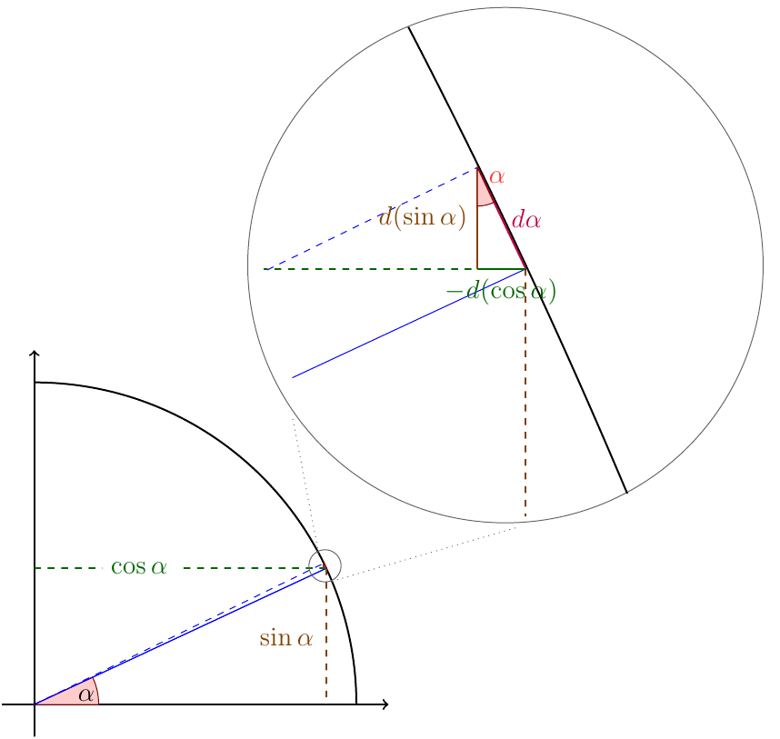
Summed up on one diagram:
Short version
By looking at how the line $\sin \alpha$ and $\cos \alpha$ change when we change $\alpha$ a little bit ($d\alpha$) and noting that we form a similar triangle, we know exactly what those lengths are.
Long version
You'll notice I've drawn a unit circle in the bottom right, chosen an angle $\alpha$, and shown both $\sin \alpha$ and $\cos \alpha$ on the plot.
We are interested in how $\sin \alpha$ changes when we make a very small change in $\alpha$, so I've done just that. I've moved the blue line from and angle of $\alpha$ to the dotted line at an angle of $\alpha + d\alpha$. Don't get caught up on the $d$ symbol here, it just means 'a little bit of'.
Since we've only moved the angle a little bit, I've included a zoomed in picture in the upper right so that we can continue. Here, we see the solid and dashed lines again where they meet our unit circle. Notice that since we've zoomed in quite a bit the circle's edge doesn't look very circley anymore, it looks like a straight line.
In fact that is the first thing we'll note, namely that the arc of the circle we trace when we change the angle a little bit has the length $d\alpha$. We know this is the case because we know that we've only gone an angle $d\alpha$, which is a small fraction $d\alpha/2\pi$ of the total circumference of the circle. The total circumference is itself $2\pi$ so at the end of the day, the length of that little bit of arc is just:
$$ \frac{ d\alpha }{2\pi} 2\pi = d\alpha $$
which we may have remembered anyway from our trig classes. What is important here is that even though $d \alpha$ is the length of the arc, when we are this zoomed in,
we can treat the arc as a straight line. In fact if we imagine taking our change $d\alpha$ smaller and smaller,
approximating the segment of arc as a line gets better and better. [Technically it should be noted that what is important is that the correction between the arc length and line length is higher order in $d\alpha$, so it can be ignored to linear order]
You'll notice that in the zoomed in picture, we can see the yellow and green segments,
which correspond to the changes in the length of the dotted yellow and green segments
from the zoomed out picture. These are the segments I've marked $d(\sin \alpha)$ and $-d(\cos \alpha)$, because the represent the change in the length of the $\sin \alpha$ line
and $\cos \alpha$ line respectively. The green segment is marked $-d(\cos \alpha)$ because the $\cos \alpha$ line actually shrinks when we increase $\alpha$ a little bit.
Now for the kicker. Notice the right triangle formed by the green, yellow and red sements? That is similar to the larger triangle in the zoomed out picture. I've marked the similar angle in red. If you stare at the picture for a bit, you can convince yourself of this fact. If all else fails, just compute all of the angles involved in the intersection of the circle with the blue line, they can all be resolved.
Knowing that the two triangles are similar, we know that the lengths of theirs sides are equal except for some scale factor, in particular:
$$ \frac{ d(\sin \alpha) }{\cos \alpha} = \frac{ d\alpha }{ 1} $$
or
$$ d(\sin \alpha) = \cos \alpha \ d\alpha $$
And we've done it! Shown the derivative of $\sin \alpha$ with a little picture.
In particular, the change in the sine of the angle ($d(\sin \alpha)$) is equal to the cosine of that angle $\cos \alpha$ times the amount we change it. In the limit of very tiny angle changes, this tells us the derivative of $\sin \alpha$:
$$ \frac{d}{d\alpha} \sin \alpha = \cos \alpha $$
Doing the same for the $d(\cos \alpha)$ segment gives
$$ d(\cos \alpha) = -\sin\alpha \ d\alpha $$
and we even get the sign right.
From here, the other trigonometric derivates are easy to obtain, either by making similar pictures al la the complete triangle,
or by using the regular rules relating all of the trigonometric function to one another.
Recently I have seen quite a few blog posts written about re-evaluating
the points values assigned to the different letter tiles in the
Scrabble™ brand Crossword Game. The premise behind these posts is that
the creator and designer of the game assigned point values to the
different tiles according to their relative frequencies of occurrence in
words in English text, supplemented by information gathered while
playtesting the game. The points assigned to different letters reflected
how difficult it was to play those letters: common letters like E, A,
and R were assigned 1 point, while rarer letters like J and Q were
assigned 8 and 10 points, respectively. These point values were based on
the English lexicon of the late 1930’s. Now, some 70 years later, that
lexicon has changed considerably, having gained many new words (e.g.:
EMAIL) and lost a few old ones. So, if one were to repeat the analysis
of the game designer in the present day, would one come to different
conclusions regarding how points should be assigned to various letters?
I’ve decided to add my own analysis to the recent development because I
have found most of the other blog posts to be unsatisfactory for a
variety of reasons[1].
One article
calculated letters’ relative frequencies by counting the number of times
each letter appeared in each word in the Scrabble™ dictionary. But this
analysis is faulty, since it ignores the probability with which
different words actually appear in the game. One is far less likely to
draw QI than AE during a Scrabble™ game (since there’s only one Q in the
bag, but many A's and E's). Similarly, very long words like
ZOOGEOGRAPHICAL have a vanishingly small probability of appearing in the
game: the A’s in the long words and the A’s in the short words cannot be
treated equally. A second article I saw calculated
letter frequencies based on their occurrence in the Scrabble™ dictionary
and did attempt to weight frequencies based on word length. The author
of this second article also claimed to have quantified the extent to
which a letter could “fit well” with the other tiles given to a player.
Unfortunately, some of the steps in the analysis of this second article
were only vaguely explained, so it isn’t clear how one could replicate
the article’s conclusions. In addition, as far as I can tell, neither of
these articles explicitly included the distribution of letters (how many
A’s, how many B’s, etc) included in a Scrabble™ game. Also, neither of
these articles accounted for the fact that there are blank tiles (that
act as wild cards and can stand in for any letter) that appear in the
game.
So, what does one need to do to improve upon the analyses already
performed? We’re given the Scrabble™ dictionary and bag of 100
tiles
with a set distribution, and we’re going to try to determine what a good
pointing system would be for each letter in the alphabet. We’re also
armed with the knowledge that each player is given 7 letters at a time
in the game, making words longer than 8 letters very rare indeed. Let’s
say for the sake of simplicity that words 9 letters long or shorter
account for the vast majority of words that are possible to play in a
normal game.
Based on these constraints, how can one best decide what points to
assign the different tiles? As stated above, the game is designed to
reward players for playing words that include letters that are more
difficult to use. So, what makes an easy letter easy, and what makes a
difficult letter difficult? Sure, the number of times the letter appears
in the
dictionary
is important, but this does not account for whether or not, on a given
rack of tiles (a rack of tiles is to Scrabble™ as a hand of cards is to
poker), that letter actually can be used. The letter needs to combine
with other tiles available either on the rack or on the board in order
to form words. The letter Q is difficult to play not only because it is
used relatively few times in the dictionary, but also because the
majority of Q-words require the player to use the letter U in
conjunction with it.
So, what criterion can one use to say how useful a particular tile is?
Let’s say that letters that are useful have more potential to be used in
the game: they provide more options for the players who draw them. Given
a rack of tiles, one can generate a list of all of the words that are
possible for the player to play. Then, one can count the number of times
that each letter appears in that list. Useful letters, by this
criterion, will combine more readily with other letters to form words
and so appear more often in the list than un-useful letters.
(I would also like to take a moment to preempt criticism from the
competitive Scrabble™ community by
saying that strategic decisions made by the players need not be brought
into consideration here. The point values of tiles are an engineering
constraint of the game. Strategic decisions are made by the players,
given the engineering constraints of the game. Words that are “available
to be played” are different from “words that actually do get played.”
The potential usefulness of individual letter tiles should reflect
whether or not it is even possible to play them, not whether or not a
player decides that using a particular group of tiles constitutes an
optimal move.)
To give an example, suppose I draw the rack BEHIWXY. I can
generate[2]
the full list of words available to be played given this rack: BE, BEY,
BI, BY, BYE, EH, EX, HE, HEW, HEX, HEY, HI, HIE, IBEX, WE, WEB, WHEY,
WHY, WYE, XI, YE, YEH, YEW. Counting the number of occurrences of each
letter, I see that the letter E appears 18 times, while the letter W
only appears 7 times. This example tells me that the letter E is
probably much more potentially useful than the letter W.
The example above is only one of the many, many possible racks that one
can see in a game of Scrabble™. I can use a
Monte Carlo-type simulation
to estimate the average usefulness of the different letters by drawing
many example racks.
Monte Carlo is a technique used to estimate
numerical properties of complicated things without explicit calculation.
For example, suppose I want to know the probability of drawing a
straight flush in poker.[3] I can calculate that probability
explicitly by using combinatorics, or I can use a Monte Carlo method to
deal a large number of hypothetical possible poker hands and count the
number of straight flushes that appear. If I deal a large enough number
of hands, the fraction of hands that are straight flushes will converge
upon the correct analytic value. Similarly here, instead of explicitly
calculating the usefulness of each letter, I use Monte Carlo to draw a
large number of hypothetical racks and use them to count the number of
times each letter can be used. Comparing the number of times that each
tile is used over many, many possible racks will give a good
approximation of how relatively useful each tile is on average. Note
that this process accounts for the words acceptable in the Scrabble™
dictionary, the number of available tiles in the bag, as well as the
probability of any given word appearing.
In my simulation, I draw 10,000,000 racks, each with 9 tiles
(representing the 7 letters the player actually draws plus two tiles
available to be played through to form longer words). I perform the
calculation two different ways: once with a 98-tile pool with no blanks,
and once with a 100-tile pool that does include blanks. In the latter
case, I make sure to not count the blanks used to stand in for different
letters as instances of those letters appearing in the game. The results
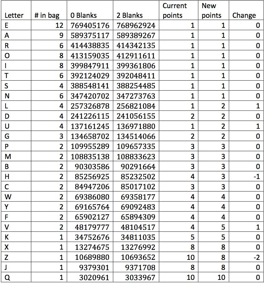
are summarized in the table below.
There are two key observations to be made here. First, it does not seem
to matter whether or not there are blanks in the bag! The results are
very similar in both cases. Second, it would be completely reasonable to
keep the tile point values as they are. Only the Z, H, and U appear out
of order. It’s only if one looks very carefully at the differences
between the usefulness of these different tiles that one might
reasonably justify re-pointing the different letters.
For fun, I have included in the table my own suggestions for what these
tiles’ values might be changed to based on the simulation results.
(Note: here's where any pretensions of scientific rigor go out the
window.) I have kept the scale of points between 1 and 10, as in the
current pointing system. I have assigned groups of letters the same
number of points based on whether they have a similar usefulness score.
Here are the significant changes: L and U, which are significantly less
useful than the other 1-point tiles may be bumped up to 2 points,
comparable to the D and G. The letter V is clearly less useful than any
of the other three 4-point tiles (W, Y, and F, all of which may be used
to form 2-letter words while the V forms no 2-letter words), and so is
undervalued. The H is comparable to the 3-point tiles, and so is
currently overvalued. Similarly, the Z is overvalued when one considers
how close to the J it is. Unlike in the previous two articles that I
mentioned, I don't find any strong reason to change the value of the
letter X compared to the other 8 point tiles. I suppose one could lower
its value from 8 points to 7, but I have (somewhat arbitrarily) chosen
not to do so.
One may also ask the question whether or not the fact that a letter
forms 2- or 3-letter words is unfairly biasing that letter. In
particular, is the low usefulness of the C and V compared to
comparably-pointed tiles due to the fact that they form no 2-letter
words? Performing the simulation again without 2-letter words, I found
no changes in the results in any of the letters except for C, which
increased in usefulness above the B and the H. The letter V's ranking,
however, did not change at all, indicating that unlike the C the V is
difficult to use even when combining with letters to make longer words.
Repeating the simulation yet again without 2- or 3-letter words yielded
the same results.
As a final note, I would like to respond directly to to Stefan Fatsis's
excellent article
about the so-called controversy surrounding re-calculating tile values
and say that I am fully aware that this is indeed a "statistical
exercise," motivated mostly by my desire to do the calculation made by
others in a way that made sense in the context of the game of Scrabble.
Similarly, I realize that these recommendations are unlikely to actually
change anything. Given that the original points values of the tiles are
still justifiably appropriate by my analysis, it's not like anybody at
Hasbro is going to jump to "fix" the game. Lastly, my calculations have
nothing to do with the strategy of the game whatsoever, and cannot be
used to learn how to play the game any better. (If anything, I've only
confirmed some things that many experienced Scrabble players already
know about the game, such as that the V is a tricky tile, or that the H,
X, and Z tiles, in spite of their high point values, are quite
flexible.)
Notes
1. ^ To state my own credentials, I have played Scrabble™competitively for
4 years, and am quite familiar with the mechanics of the game, as well
as contemporary strategy.
2. ^ Credit where credit is due: Alemi provided the code used to
generate the list of available words given any set of tiles. Thanks
Alemi!
3. ^ Monte Carlo has a long history of being used to estimate the
properties of games. As recounted by George Dyson in Turing’s
Cathedral, in 1948 while at Los Alamos the mathematician Stanislaw Ulam
suffered a severe bout of encephalitis that resulted in an emergency
trepanation. While recovering in the hospital, he played many games of
solitaire and was intrigued by the question of how to calculate the
probability that a given deal could result in a winnable game. The
combinatorics required to answer this question proved staggeringly
complex, so Ulam proposed the idea of generating many possible solitaire
deals and merely counting how many of them resulted in victory. This
proved to be much simpler than an explicit calculation, and the rest is
history: Monte Carlo is used today in a wide variety of applications.
Additional References:
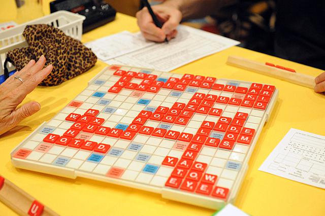
The photo at top of a Scrabble™ board was taken during the 2012 National
Scrabble™ Championship. Check out the 9-letter double-blank BINOCULAR.
For anyone interested in learning more about the fascinating world of
competitive Scrabble™, check out Word Freak, also by Stefan Fatsis.
This book has become more or less the definitive documentation upon this
subculture. If you don't have enough time to read, check out Word
Wars, a documentary that
follows many of the same people as Fatsis's book. (It still may be
available streaming on Netflix if you hurry.)
A lot of the research I’m interested in relates to networks – measuring
the properties of networks and figuring out what those properties mean.
While doing some background reading, I stumbled upon some discussion of
the algorithm that search engines use to rank search results. The
automatic ranking of the results that come up when you search for
something online is a great example of how understanding networks (in
this case, the World Wide Web) can be used to turn a very complicated
problem into something simple.
Ranking search results relies on the assumption that there is some
underlying pattern to how information is organized on the WWW- there are
a few core websites containing the bulk of the sought-after information
surrounded by a group of peripheral websites that reference the core.
Recognizing that the WWW is a network representation of how information
is organized and using the properties of the network to detect where
that information is centered are the key components to figuring out what
websites belong at the top of the search page.
Suppose you look something up on Google (looking for YouTube videos of
your favorite band, looking for edifying science
writing, tips on octopus pet care,
etc): the search service returns a whole spate of results. Usually, the
pages that Google recommends first end up being the most useful. How on
earth does the search engine get it right?
First I’ll tell you exactly how Google does not work. When you type in
something into the search bar and hit enter, a message is not sent to
a guy who works for Google about your query. That guy does not then
look up all of the websites matching your search, does not visit each
website to figure out which ones are most relevant to you, and does
not rank the pages accordingly before sending a ranked list back to
you. That would be a very silly way to make a search engine work! It
relies on an individual human ranking the search results by hand with
each search that’s made. Maybe we can get around having to hire
thousands of people by finding a clever way to automate this process.
So here’s how a search engine does work. Search engines use robots
that crawl around the World Wide Web (sometimes these robots are
referred to as “spiders”) finding websites, cataloguing key words that
appear on those webpages, and keeping track of all the other sites that
link into or away from them. The search engine then stores all of these
websites and lists of their keywords and neighbors in a big database.
Knowing which websites contain which keywords allows a search engine to
return a list of websites matching a particular search. But simply
knowing which websites contain which keywords is not enough to know how
to order the websites according to their relevance or importance.
Suppose I type “octopus pet care” into Google. The search yields 413,000
results- far too many for me to comb through at random looking for the
web pages that best describe what I’m interested in.
Knowing the ways that different websites connect to one another through
hyperlinks is the key to how search engine rankings work. Thinking of a
collection of websites as an ordinary list doesn’t say anything about
how those websites relate to one another. It is more useful to think of
the collection of websites as a network, where each website is a node
and each hyperlink between two pages is a directed edge in the network.
In a way, these networks are maps that can show us how to get from one
website to another by clicking through links.
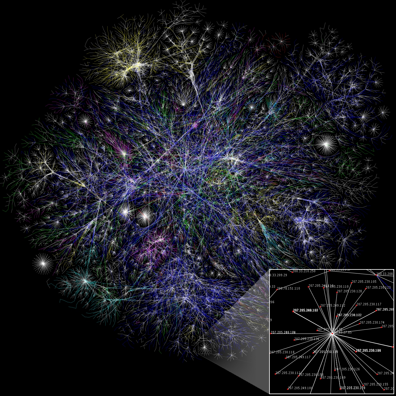
Here is an example of what a network visualization of a website map of a
large portion of the WWW looks like. (Original full-size image
here.)
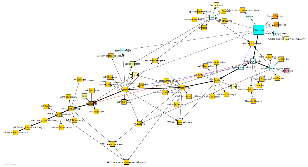
Here is a site map for a group of websites that connect to the main page
of English Wikipedia. (Original image from
here.) This smaller site map is
closer to the type of site map used when making a search using a search
engine.
So, how does knowing the underlying network of the search results help
one to find the best website on octopus care (or any other topic)? The
search engine assumes that behind the seemingly random, hodgepodge
collection of files on the WWW, there is some organization in the way
they connect to one another. Specifically, the search engine assumes
that finding the websites most central to the network of search results
is the same as finding the search results with the best information.
Think of a well-known, trusted source of information, like the New York
Times. The NY Times website will have many other websites referencing it
by linking to it. In addition, the NY Times website, being a trusted
news source, is likely to refer to the best references for other sources
that it wants to refer to, such as Reuters. High-quality references will
also probably have many incoming links from websites that cite them. So
not only does a website like the NY Times sit at the center of many
other websites that link to it, but it also frequently connects to other
websites that themselves are at the center of many other websites. It is
these most central websites that are probably the best ones to look at
when searching for information.
When I search for “octopus pet care” using Google I am necessarily
assuming that the search results are organized according to this
core-periphery structure, with a group of important core websites
central to the network surrounded by many less important peripheral
websites that link to the core nodes. The core websites may also connect
to one another. There may also be websites disconnected from the rest,
but these will probably be less important to the search simply because
of the disconnection. Armed with the knowledge of the connections
between the different relevant websites and the core-periphery network
structure assumption, we may now actually find which of the websites are
most central to the network (in the core), and therefore determine which
websites to rank highly.
Let’s begin by assigning a quantitative “centrality” score to each of
the nodes (websites) in the network, initially guessing that all of the
search results are equally important. (This, of course, is probably not
true. It’s just an initial guess.) Each node then transfers all of its
centrality score to its neighbors, dividing it evenly between
them[1].
(Starting with a centrality score of 1 with three neighbors, each of
those neighbors receives 1/3.) Each node also receives a some centrality
from each neighbor that links in to it. Following this first step, we
find that nodes with many incoming edges will have higher centrality
than nodes with few incoming edges. We can repeat this process of
dividing and transferring centrality again. Nodes with many incoming
links will have more centrality to share with their neighbors, and nodes
with many incoming links will themselves also receive more centrality.
After repeating this process many times, we begin to see a difference
between which nodes have the highest centrality scores: nodes with high
centrality are the ones that have many incoming links, or have links to
other central nodes, or both. This algorithm therefore differentiates
between the periphery and the core of the network. Core nodes receive
lots of centrality because they link to one another and because they
have lots of incoming links from the periphery. Peripheral nodes have
fewer incoming links and so receive less centrality than the nodes in
the core. Knowing the centrality scores of search results on the WWW
makes it pretty straightforward for us to quantitatively rank which of
those websites belongs at the top of the list.
Of course, there are more complex ways that one can add to and improve
this procedure. Google’s algorithm PageRank (named for founder Larry
Page, not because it is used to rank web pages) and the HITS algorithm
developed at Cornell are two examples of more advanced ways of ranking
search engine results. We can go even further: a search engine can keep
track of the links that users follow whenever a particular search is
made. (This is almost the same as the company hiring someone to order
sought-after web pages automatically whenever a search is made, except
all the company lets the user do it for free.) Over time, search engines
can improve their methods for helping us find what we need by learning
directly from the way users themselves prioritize which search results
they pursue. Still, these different search engine ranking systems may
operate using slightly different methods, but all of them depend on
understanding the list of search results within the context of a
network.
Notes
1. ^ It's not always all - there are other variations where nodes only
transfer a fraction of their centrality score at each step.
Sources (and further reading)
I wanted to include no mathematics in
this post simply because I cannot explain the mathematics behind these
algorithms and their convergence properties better than my sources can.
For those of you who want to see the mathematical side of the argument
for yourselves (which involves treating the network adjacency matrix as
a Markov process and finding its nontrivial steady state eigenvector),
do consult the following two textbooks:
Easley, David, and Jon Kleinberg. Networks, Crowds, and Markets:
Reasoning about a Highly Connected World. Cambridge University Press,
2010 (Chapter 14
in particular)
Newman, Mark. Networks: an Introduction. Oxford
University Press, 2010 (Chapter 7 in particular)
A popular book on the early development of network science that contains
a lot of information on the structure of the WWW:
Barabasi, Albert-Laszlo. Linked: How Everything is Connected to
Everything Else and What It Means. Plume, 2003.
A book on the history of modern computing that contains an interesting
passage on how search engines learn adaptively from their users (that
deserves a shout-out in this blog post).
The time I spent making this poster could have been spent doing research
Since December 2012 is coming up, I thought I'd help the Mayans out with
a look at a possible end of the world scenario. (I know, it's not Earth
Day yet, but we at the Virtuosi can only go so long without fantasizing
about wanton destruction.) As the Earth zips around the Sun, it moves
through the heliosphere,
which is a collection of charged particles emitted by the Sun. Like any
other fluid, this will exert drag on the Earth, slowly causing it to
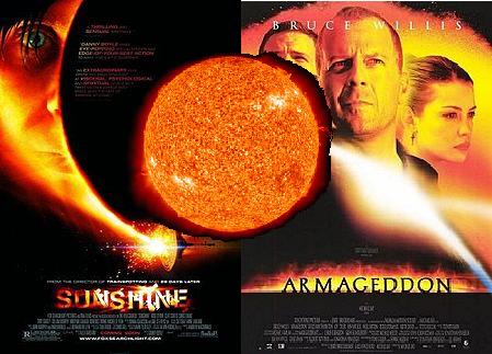
spiral into the Sun. Eventually, it will burn in a blaze of glory, in a
bad-action-movie combination of Sunshine meets Armageddon. Before I get
started, let me preface this by saying that I have no idea what the hell
I'm talking about. But, in the spirit of being an arrogant physicist,
I'm going to go ahead and make some back-of-the-envelope calculations,
and expect that this post will be accurate to within a few orders of
magnitude. Well, how long will the Earth rotate around the Sun before
drag from the heliosphere stops it? This seems like a problem for fluid
dynamics. How do we calculate what the drag is on the Earth? Rather than
solve the fluid dynamics equations, let's make some arguments based on
dimensional analysis. What can the drag of the Earth depend on? It
certainly depends on the speed of the Earth v -- if an object isn't
moving, there can't be any drag. We also expect that a wider object
feels more drag, so the drag force should depend on the radius of the
Earth R. Finally, the density of the heliosphere might have something to
do with it. If we fudge around with these, we see that there is only 1
combination that gives units of force:
$$ F_{drag} \sim \rho v^2 R^2 $$
Now that we have the force, the energy dissipated from the Earth
to the heliosphere after moving a distance $d$ is $E_\textrm{lost} = F\times d$. If
the Earth moves with speed v for time t, then we can write
$E_\textrm{lost} = F v t$. So we can get an idea of the time scale over which the Earth
starts to fall into the Sun by taking
$E_\textrm{lost} = E_\textrm{Earth} \sim 1/2 M_\textrm{Earth} v^2$.
Rearranging and dropping factors of 1/2 gives
Using the velocity of the Earth as $2\pi \times 1 \mbox{Astronomical unit/year}$,
Googlin' for some numbers, and taking the
density of the heliosphere
to be $10^{-23}$ g/cc we get...
$$ T \approx 10^{19} \textrm{ years} $$
Looks like this won't be the cause of the Mayan apocalypse. (By comparison, the
Sun will burnout
after only $\sim10^9$ years.)
A while ago I decided I wanted to create something that looks like the
surface of a planet, complete with continents & oceans and all. Since
I've only been on a small handful of planets, I decided that I'd
approximate this by creating something like the Earth on the computer
(without cheating and just copying the real Earth). Where should I
start? Well, let's see what the facts we know about the Earth tell us
about how to create a new planet on the computer.
Observation 1:
Looking at a map of the Earth, we only see the heights of the surface.
So let's describe just the heights of the Earth's surface.
Observation 2:
The Earth is a sphere. So (wait for it) we need to describe the
height on a spherical surface. Now we can recast our problem of making
an Earth more precisely mathematically. We want to know the heights of
the planet's surface at each point on the Earth. So we're looking for
field (the height of the planet) defined on the surface of a sphere (the
different spots on the planet). Just like a function on the real line
can be expanded in terms of its Fourier components, almost any function
on the surface of a sphere can be expanded as a sum of spherical
harmonics $Y_{lm}$. This means we can write the height $h$ of our planets
surfaces as
If we figure out what the coefficients $A$ of the sum should
be, then we can start making some Earths! Let's see if we can use some
other facts about the Earth's surface to get get a handle on what
coefficients to use.
Observation 3:
I don't know every detail of the Earth's surface, whose history
is impossibly complicated. I'll capture
this lack-of-knowledge by describing the surface of our imaginary planet
as some sort of random variable. Equation (1) suggests that we can do
this by making the coefficients $A$ random variables. At some point we
need to make an executive decision on what type of random variable we'll
use. For various reasons,[1]
I decided I'd use a Gaussian
random variable with mean 0 and standard deviation $a_{lm}$:
$$ A_{lm} = a_{lm} N(0,1) $$
(Here I'm using the notation that $N(m,v)$ is a normal
or Gaussian random variable with mean $m$ and variance $v$. If you
multiply a Gaussian random variable by a constant $a$, it's the same as
multiplying the variance by $a^2$, so $a N(0,1)$ and $N(0,a^2)$ are
the same thing.)
Observation 4:
The heights of the surface of the
Earth are more-or-less independent of their position on the Earth. In
keeping with this, I'll try to use coefficients $a_{lm}$ that will give me
a random field that is is isotropic on average. This seems hard at
first, so let's just make a hand-waving argument. Looking at some
pretty pictures
of spherical harmonics, we can see that each spherical harmonic of degree $l$
has about $l$ stripes on it, independent of $m$.
So let's try using $a_{lm}$'s
that depend only on $l$, and are constant if just
$m$ changes[2]. Just for convenience,
we'll pick this constant to be $l$ to some power $-p$:
At this point I got bored & decided to see what a
planet would look like if we didn't know what value of $p$ to use. So
below is a movie of a randomly generated "planet" with a fixed choice of
random numbers, but with the power $p$ changing.
As the movie starts ($p=0$), we see random uncorrelated heights on the
surface.[3] As the movie continues and $p$ increases, we see
the surface smooth out rapidly. Eventually, after $p=2$ or so, the planet
becomes very smooth and doesn't look at all like a planet. So the
"correct" value for p is somewhere above 0 (too bumpy) and below 2 (too
smooth). Can we use more observations about Earth to predict what a good
value of $p$ should be?
Observation 5:
The elevation of the Earth's
surface exists everywhere on Earth (duh). So we're going to need our sum
to exist. How the hell are we going to sum that series though! Not only
is it random, but it also depends on where we are on the planet! Rather
than try to evaluate that sum everywhere on the sphere, I decided that
it would be easiest to evaluate the sum at the "North Pole" at
$\theta=0$. Then, if we picked our coefficients right, this should be
statistically the same as any other point on the planet. Why do we want
to look at $\theta = 0$? Well, if we look back at the
wikipedia entry
for spherical harmonics, we see that
That doesn't look too helpful -- we've just picked up
another special function $P_l^m$ that we need to worry about. But there is a
trick with these special functions $P_l^m$: at $\theta = 0$, $P_l^m$ is 0 if $m$
isn't 0, and $P_l^0$ is 1. So at $\theta = 0$ this is simply:
So for the surface of our imaginary planet to exist, we had better have that sum
converge, or $-2p+1 < -1 ~ (p > 1)$. And we've also learned something
else!!! Our model always gives back a Gaussian height distribution on
the surface. Changing the coefficients changes the variance of
distribution of heights, but that's all it does to the distribution.
Evidently if we want to get a non-Gaussian distribution of heights, we'd
need to stretch our surface after evaluating the sum. Well, what does
the height distribution look like from my simulated planets? Just for
the hell of it, I went ahead and generated ${\sim}400$ independent surfaces at
${\sim}40$ different values for the exponent $p$, looking at the first 22,499
terms in the series. From these surfaces I reconstructed the measured
distributions; I've combined them into a movie which you can see below.
As you can see from the movie, the distributions look like Gaussians.
The fits from Eq. (4) are overlaid in black dotted lines. (Since I can't
sum an infinite number of spherical harmonics with a computer, I've
plotted the fit I'd expect from just the terms I've summed.) As you can
see, they are all close to Gaussians. Not bad. Let's see what else we
can get.
Observation 6:
According to some famous people, the Earth's surface is
probably a fractal
whose coastlines are non-differentiable.
This means that we want a value of $p$ that will make our surface rough
enough so that its gradient doesn't exist (the derivative of the sum of
Eq. (2) doesn't converge). At this point I'm getting bored with writing
out calculations, so I'm just going to make some scaling arguments. From
Eq. (3), we know that each of the spherical harmonics $Y_l^m$ is related to
a polynomial of degree $l$ in $\cos \theta$. So if we take a derivative, I'd
expect us to pick up another factor of $l$ each time. Following through
all the steps of Eq. (4) we find
which converges for $p > 2$. So for our planet to be "fractal," we want $1<p<2$.
Looking at the first movie, this seems reasonable.
Observation 7:
70% of the Earth's surface is under water. On Earth, we can think of the points
underwater as all those points below a certain threshold height. So
let's threshold the heights on our sphere. If we want 70% of our
generated planet's surface to be under water, Eq (4) and the
cumulative distribution function
of a
Gaussian distribution
tells us that we want to pick a critical height $H$ such that
where $\textrm{erf}()$ is a special function called the error function,
and $\textrm{erf}^{-1}$ is its inverse. We can evaluate these numerically (or by using some
dirty tricks
if we're feeling especially masochistic). So for our generated planet,
let's call all the points with a height larger than $H$ "land," and all
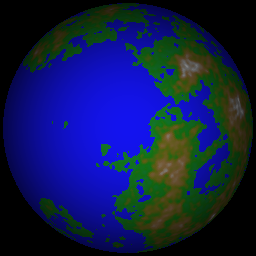
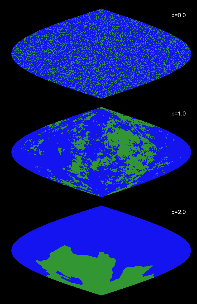
the points with a height less than $H$ "ocean." Here is what it looks like
for a planet with $p=0$, $p=1$, and $p=2$, plotted with the same
Sanson projection
as before.
Top to bottom: p=0, p=1, and p=2. I've colored all the "water" (positions with heights < $H$ as given in Eq. (5) ) blue and all the land (heights > $H$) green.
You can see that the the total amount of land area is roughly constant
among the three images, but we haven't fixed how it's distributed.
Looking at the map above for $p=0$, there are lots of small "islands"
but no large contiguous land masses. For $p=2$, we see only one
contiguous land mass (plus one 5-pixel island), and $p=1$ sits somewhere
in between the two extremes. None of these look like the Earth, where
there are a few large landmasses but many small islands. From our
previous arguments, we'd expect something between $p=1$ and $p=2$ to look
like the Earth, which is in line with the above picture. But how do we
decide which value of p to use?
Observation 8:
The Earth has 7 continents This one is more vague than the others, but I think it's the
coolest of all the arguments. How do we compare our generated planets to
the Earth? The Earth has 7 continents that comprise 4 different
contiguous landmasses. In order, these are 1) Europe-Asia-Africa, 2)
North- and South- America, 3) Antartica, and 4) Australia, with a 5th
Greenland barely missing out. In terms of fractions of the Earth's
surface, Google tells us that Australia covers 0.15% of the Earth's
total surface area, and Greenland covers 0.04%. So let's define a
"continent" as any contiguous landmass that accounts for more than 0.1%
of the planet's total area. Then we can ask: What value of p gives us
a planet with 4 continents? I have no idea how to calculate exactly what
that number would be from our model, but I can certainly measure it from
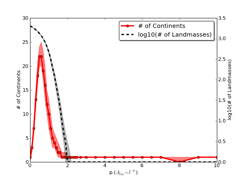
the simulated results. I went ahead and counted the number of continents
in the generated planets.
The results are plotted above. The solid red line is the median values
of the number of continents, as measured over 400 distinct worlds at 40
different values of $p$. The red shaded region around it is the band
containing the upper and lower quartiles of the number of continents.
For comparison, in black on the right y-axis I've also plotted the log
of the total number of landmasses at the resolution I've used. The
number of continents has a resonant value of $p$ -- if $p$ is too small,
then there are many landmasses, but none are big enough to be
continents. Conversely, if $p$ is too large, then there is only one huge
landmass. Somewhere in the middle, around $p=0.5$, there are about 20
continents, at least when only the first ${\sim}23000$ terms in the series are
summed. Looking at the curve, we see that there are roughly two places
where there are 4 continents in the world -- at $p=0.1$ and at $p=1.3$.
Since $p=0.1$ doesn't converge, and since $p=0.1$ will have way too many
landmasses, it looks like a generated Earth will look the best if we use
a value of $p=1.3$ And that's it.
For your viewing pleasure, here is a video of three of these planets below,
complete with water, continents, and mountains.[4]
Notes
1. ^ Since I wanted a random surface, I wanted to make the mean of each
coefficient 0. Otherwise we'd get a deterministic part of our surface
heights. I picked a distribution that's symmetric about 0 because on
Earth the bottom of the oceans seem roughly similar in terms of changes
in elevation. I wanted to pick a stable distribution & independent
coefficients because it makes the sums that come up easier to evalutate.
Finally, I picked a Gaussian, as opposed to another stable distribution
like a Lorentzian, because the tallest points on Earth are finite, and I
wanted the variance of the planet's height to be defined.
2. ^ We could make this rigorous by showing that a rotated spherical
harmonic is orthogonal to other spherical harmonics of a different
degree $l$, but you don't want to see me try.
3. ^ Actually $p=0$ should correspond to completely uncorrelated
delta-function noise. (You can convince yourself by looking at the
spherical harmonic expansion for a delta-function.) The reason that the
bumps have a finite width is that I only summed the first 22,499 terms
in the series ($l=150$ and below). So the size of the bumps gives a rough
idea of my resolution.
4. ^ For those of you keeping score at home, it took me more than 6 days
to figure out how to make these planets.
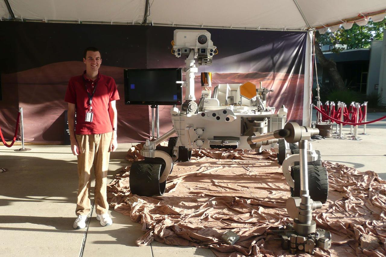
In less than two days, NASA's Mars Science Laboratory (MSL) / Curiosity
rover will begin its harrowing descent to the Martian
surface. If everything goes according to the
kind-of-crazy-what-the-heck-is-a-sky-crane plan, this process will be
referred to as "landing" (otherwise, more crashy/explodey gerunds will
no doubt be used). The MSL mission is run through NASA's Jet Propulsion
Laboratory where, by coincidence, I happen to be at the moment. Now, I'm
not working on this project, so I don't have a lot to add that
isn'tavailableelsewhere.
BUT I do feel an authority-by-proximity kind of fallacy kicking in, so
how about a post why not?
Preliminaries
Before we get started, I feel obligated to link to NASA's
Seven Minutes of Terror
video. If you haven't seen it yet, I highly recommend watching it right now (my
favorite part is the subtitles). It has over a million views on YouTube
and seems to have done a pretty good job at generating interest in the
mission. Although, it's a shame they had to interview the first guy in
what appears to be a police interrogation room. Oh well.
About the Rover
This thing is big. It's the size of a car and is jam-packed with
scientific equipment.
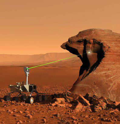
There's a couple different spectrometers, a bunch of cameras, a drill for
collecting rock samples, and radiation detectors. Probably the coolest
instrument onboard Curiosity is called the ChemCam. The ChemCam uses a
laser to vaporize small regions of rock, which allows it to study the
composition of things about 20 feet away.
In addition to the scientific payload, Curiosity also needs some way
to generate power. Previous rovers had been powered by solar panels, but
there don't appear to be any here. Instead, Curiosity is
powered
by the heat released from the radioactive decay of about 10 pounds of plutonium
dioxide. This source will power the rover for
about a Martian year
well beyond the currently planned mission duration of one Martian year
(about 687 Earth days) [Thanks to Nathan in the comments for pointing
this out!].
To summarize, the rover is a nuclear-powered lab-on-wheels that
shoots lasers out of its head. This is pretty cool.
In non-SI units, the MSL is roughly one handsome man (1 hm) tall
A Curious Footprint
There's been a lot of preparation at JPL this week for the upcoming
landing. All the shiny rover models have been taken out of the visitor's
center and put in a tent outside, presumably so there will be a pretty
backdrop for press reports and the like.
Anyway, I was out taking pictures of the rovers at the end of the day
today when someone pointed out something cool about the tires on
Curiosity.
Here's a close-up:
Hole-y Tires
Each tire on the rover is has "JPL" punched out in
Morse code!
Makes sense, though. If you're going to spend $2.5 billion on something,
you might as well put your name on it.
Watch the Landing
If you want to watch the landing, check out the
NASA TV stream.
The landing is scheduled for Sunday night at 10:31 pm PDT (1:31 am EDT). Until then,
it looks like they are showing a lot of interviews and other cool
behind-the-scenes kind of stuff.


