 I was rather proud of my last post about being caught in the
rain. In
that post, I concluded that you were better off running in the rain, but
that the net effect wasn't incredibly great. However, when I told people
about it, the question I inevitably got asked was: What if the rain
isn't vertical? That's what I'd like to look at today, and it turns out
to be a much more challenging question. I'm still going to assume that
the rain is falling at a constant rate. Furthermore, I'm going to assume
that the angle of the rain doesn't change. With those two assumptions
stated, let me remind you of the definitions we used last time. $$\rho
- \text{the density of water in the air in liters per cubic meter}$$
$$A_t - \text{top area of a person}$$ $$\Delta t - \text{time
elapsed}$$ $$d - \text{distance we have to travel in the rain}$$ $$v_r
- \text{raindrop velocity}$$ $$A_f - \text{front area of a person}$$
$$W_{tot} - \text{total amount of water in liters we get hit with}$$
As a reminder, our result from last time was: $$W_{tot}= \rho d (A_t
\frac{v_r}{v} + A_f)$$ Now, let's look at the new analysis. As
before, let us consider the stationary state first. Our velocity now has
two components, horizontal and vertical. Analogous to the purely
vertical situation, we can write down the stationary state, but now we
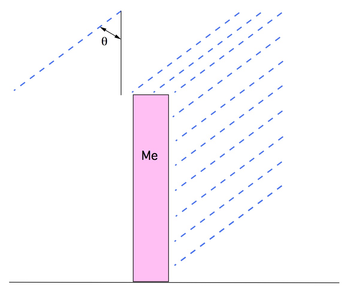
have rain hitting both our top and front (or back). I'm going to define
the angle, theta, as the angle the rain makes with the vertical (check
out figure 1 below). this gives $$W = \rho d A_t v_r \cos(\theta)
\Delta t+\rho A_f v_r \sin(\theta) \Delta t$$ Let's check our
limits. As theta goes to zero (vertical rain), we only get rain on top
of us, and as theta goes to 90 (horizontal rain), we only get rain on
the front of us. Makes sense! Alright, so let's add in the effect of
motion now. This is going to be more challenging than in the vertical
rain situation. We're going to examine two separate cases
I was rather proud of my last post about being caught in the
rain. In
that post, I concluded that you were better off running in the rain, but
that the net effect wasn't incredibly great. However, when I told people
about it, the question I inevitably got asked was: What if the rain
isn't vertical? That's what I'd like to look at today, and it turns out
to be a much more challenging question. I'm still going to assume that
the rain is falling at a constant rate. Furthermore, I'm going to assume
that the angle of the rain doesn't change. With those two assumptions
stated, let me remind you of the definitions we used last time. $$\rho
- \text{the density of water in the air in liters per cubic meter}$$
$$A_t - \text{top area of a person}$$ $$\Delta t - \text{time
elapsed}$$ $$d - \text{distance we have to travel in the rain}$$ $$v_r
- \text{raindrop velocity}$$ $$A_f - \text{front area of a person}$$
$$W_{tot} - \text{total amount of water in liters we get hit with}$$
As a reminder, our result from last time was: $$W_{tot}= \rho d (A_t
\frac{v_r}{v} + A_f)$$ Now, let's look at the new analysis. As
before, let us consider the stationary state first. Our velocity now has
two components, horizontal and vertical. Analogous to the purely
vertical situation, we can write down the stationary state, but now we
have rain hitting both our top and front (or back). I'm going to define
the angle, theta, as the angle the rain makes with the vertical (check
out figure 1 below). this gives $$W = \rho d A_t v_r \cos(\theta)
\Delta t+\rho A_f v_r \sin(\theta) \Delta t$$ Let's check our
limits. As theta goes to zero (vertical rain), we only get rain on top
of us, and as theta goes to 90 (horizontal rain), we only get rain on
the front of us. Makes sense! Alright, so let's add in the effect of
motion now. This is going to be more challenging than in the vertical
rain situation. We're going to examine two separate cases
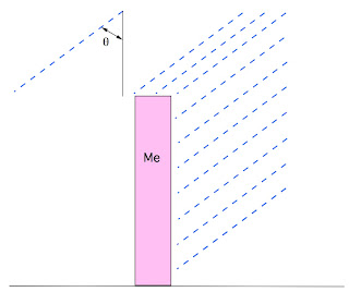 Fig. 1 - The rain, and our angle.
Case 1: Running Against The Rain This is the easier of the two
cases. After thinking about it for a while, I believe that it is the
same as when the rain is vertical. Let me explain why. If you are moving
with some velocity v, in a time t you will cover a distance x=vt. Now,
suppose we paused the rain, so it is no longer moving, then moved you a
distance x, turned the rain back on, and had you wait for a time t. And
repeated this over and over until you got to where you were going. This
would result in an average velocity equal to v, even though it is not
a smooth motion. However, my claim is that in the limit that t and x go
to zero, this is a productive way of considering our situation. We note
that v=x/t, and in the limit that both x and t go to zero, that is the
definition* of instantaneous velocity. The recap is, that my 'pausing
the rain' scheme of thinking about things is fine, as long as we
consider moving ourselves only very small distances over very short
times. Using this construction, we have an additional amount of rain
absorbed by moving the distance delta x of:
$$ \Delta W = \rho A_f \Delta x $$
$$ \Delta W = \rho A_f v \Delta t $$
This gives a net expression of
$$\Delta W = \rho A_t v_r \cos(\theta) \Delta t+\rho A_f v_r
\sin(\theta) \Delta t+\rho A_f v \Delta t $$
$$\Delta W = \rho A_f v \Delta t \left( \left(
\frac{A_t}{A_f}\right)
\left(\frac{v_r}{v}\right)\cos(\theta)+\left(\frac{v_r}{v}\right)\sin(\theta)
+ 1 \right)$$
As before, turning the deltas into differentials and integrating yields
$$W = \rho A_f v t \left( \left( \frac{A_t}{A_f} \right)
\left(\frac{v_r}{v}\right)\cos(\theta)+\left(\frac{v_r}{v}\right)\sin(\theta)
+ 1\right)$$
$$W=\rho A_f d \left( \left( \frac{A_t}{A_f}\right)
\left(\frac{v_r}{v}\right)\cos(\theta)+
\left(\frac{v_r}{v}\right)\sin(\theta) + 1 \right)$$
Note that when theta is zero, our vertical rain result gives the same
thing as we found in the last post (the first term lives, the second
term goes to zero, the third term lives). I'm going to use the
reasonable numbers I came up with in the last post. However, since we
have wind, we'll have to modify our rain velocity. More specifically,
we'll assume the rain has the same vertical component of velocity in all
cases. Then the wind speed, v_w, will be what controls the angle. More
exactly, the magnitude of the raindrop velocity will be
$$v_r=\sqrt{(6 m/s)^2+v_w^2}$$
While the angle will be
$$\theta=\tan^{-1}(v_w/ (6 m/s))$$
Next we note that
$$v_r\cos\theta = 6 m/s$$
which is just the vertical component of our rain. Similarly, the other
term is just the horizontal component of our rain. So we can write our
as a function of our velocity and the wind speed (the angle and wind
speed is interchangeable):
$$W = \rho A_f d\left( \left( \frac{A_t}{A_f}\right)
\left(\frac{6 m/s}{v}\right) +\left(\frac{v_w}{v}\right) +
1\right)$$
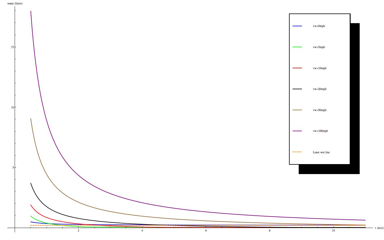
Using the reasonable numbers I came up with in my last post yields (with
a distance of 100m)
$$W = .2 liters \left( \left(\frac{.72
m/s}{v}\right)&+\left(\frac{v_w}{v}\right) + 1\right)$$
Once again, we have a least wet asymptote, which is the same as before.
I've plotted this function for various values of theta, and, more
intuitively, for various wind speeds (measured in mph, as we're used to
here in the US), and the plots are shown below (click to enlarge).
Unsurprisingly, you get the most wet when the rain is near horizontal,
but interestingly enough you can get the most percentage change from a
walk to a run when the rain is near horizontal. All angles are in
degrees.
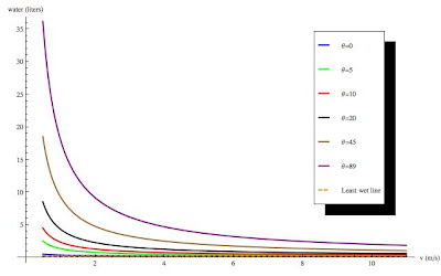 Fig. 2 - How wet you get vs. how fast you run for various wind angles.
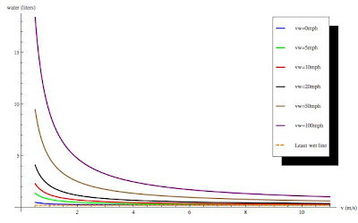 Fig. 3 - How wet you get vs. how fast you run for various wind speeds in mph.
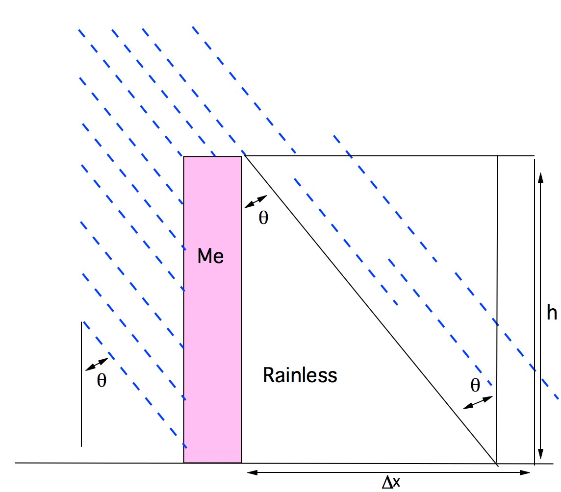
Case 2: Running With The Rain
This is the potentially harder case. We've got two obvious limiting
cases. If you run with the exact velocity of the rain and the rain is
horizontal, you shouldn't get wet. If the rain is vertical, it should
reduce to the result from my first post. We'll start with the stationary
case. This should be identical to case 1, if you're stationary it
doesn't matter if the rain is blowing on your front or back. That means
that for v=0, we should have $$\Delta W = \rho A_t v_r
\cos(\theta) \Delta t + \rho A_f v_r \sin(\theta) \Delta t$$
Now, let's use the same method as before, pausing the rain, advancing in
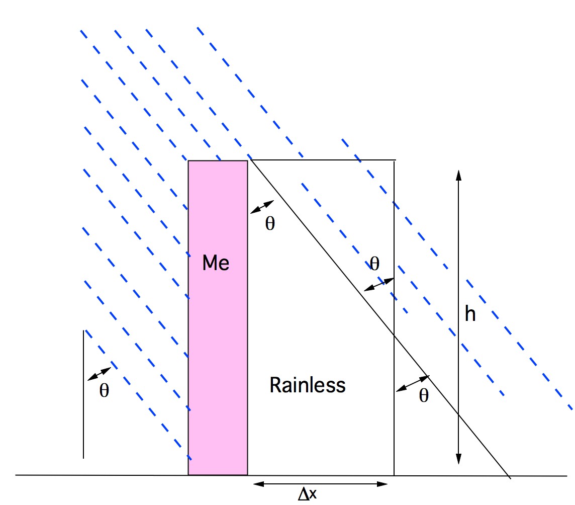
x, then letting time run. First we'll deal with our front side. Consider
figure 4.
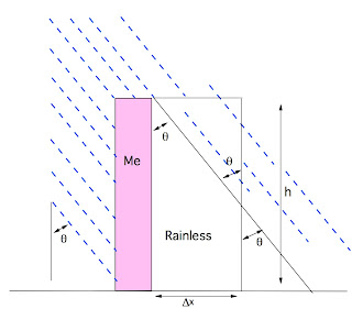 Fig. 4 - Geometry for small delta x.
Note that in front of us there is a rainless area, which we'll be
advancing into. Consider a delta x less than the length of the base of
that triangle. If we advance that delta x, we'll carve out a triangle of
rain as indicated, which, by some simple geometry, contains an amount of
rain $$\rho w \frac{(\Delta x)^2}{2 \tan(\theta)} = \rho w
\frac{v^2 (\Delta t)^2}{2 \tan(\theta)}$$ where w is the width of
our front. Now, consider if delta x is longer than the base of the
rainless triangle, as shown in figure 5.
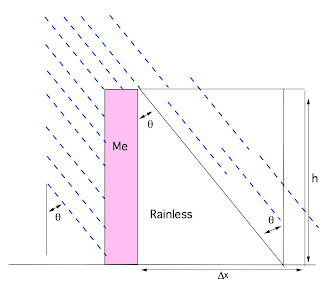 Fig. 5 - Geometry for large delta x.
We'll carve out an amount of rain equal to the indicated triangle plus
the rectangle. From the diagram we see this gives an amount of water
$$A_f \rho (\Delta x - h \tan(\theta)) + A_f \rho h
\tan(\theta)/2 = A_f \rho (\Delta x - \frac{h
\tan(\theta)}{2})$$ We could write two separate equations for these
two cases, but that's rather inefficient notation. I'm going to use the
Heaviside step
function, H(x).
This is a function that is zero whenever the argument is negative, and 1
whenever the argument is positive. That means that for our front side,
$$\Delta W_f=\rho w \frac{v^2 (\Delta t)^2}{2 \tan(\theta)} H(
h\tan(\theta) - \Delta x) $$ $$+A_f \rho \left(\Delta x -
\frac{h \tan(\theta)}{2}\right)H(\Delta x - h \tan(\theta))$$
Note that I've written my step function in terms of the relative length
of delta x and the base of the rainless triangle. We get the first term
when delta x is less than the base length, and the second term when
delta x is more than the base length. Now, let us consider the rain
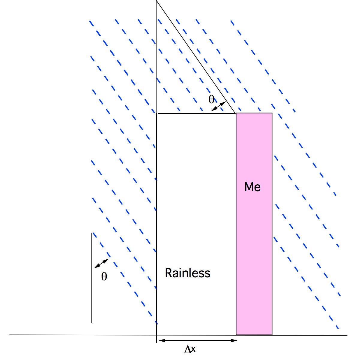
hitting our back. There are two cases here as well. First consider the
case where we're running with a velocity less than that of the rain. See
figure 6..
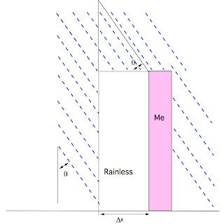 Fig. 6 - The back.
We get two terms. There's the triangle of rain that moves down and hits
our back, shown above. Hopefully it is apparent that this is the same as
the triangle of rain we carved out with our front, and so will
contribute a volume of water $$\rho w \frac{v^2 (\Delta t)^2}{2
\tan(\theta)}$$ There's also the rain that manages to catch up with
us, $$A_f \rho (v_r \sin(\theta) \Delta t - \Delta x) =A_f \rho
\Delta t (v_r \sin(\theta) - v)$$ In the case where we outrun the
rain, we don't want this term, and our triangle gains a maximal length
of the horizontal and vertical components of the rain velocity times
delta t. We can write this backside term using a step function as
$$\Delta W_b =A_f \rho \Delta t \left(v_r \sin(\theta) - v +w
\frac{v^2 (\Delta t)^2}{2 \tan(\theta)}\right)H( v_r
\sin(\theta) - v)$$ $$+\rho w v_r^2 \Delta t^2
\frac{\sin(\theta)\cos(\theta)}{2} H(v-v_r\sin(\theta))$$ We can
combine these terms, with our usual top term, to get $$\Delta W =A_f
\rho \Delta t \left[ \left(v_r \sin(\theta) - v +\frac{w}{A_f}
\frac{v^2 (\Delta t)}{2 \tan(\theta)}\right)H(v_r \sin(\theta)
- v)$$ $$+ \frac{w}{A_f} v_r^2 \Delta t
\frac{\sin(\theta)\cos(\theta)}{2} H(v-v_r\sin(\theta) $$ $$+
\frac{w}{A_f} \frac{v^2 (\Delta t)}{2 \tan(\theta)} H(
h\tan(\theta) - \Delta x)$$ $$+\left(\frac{\Delta x}{\Delta t} -
\frac{h \tan(\theta)}{2 \Delta t}\right)H(\Delta x - h
\tan(\theta))+\frac{A_t}{A_f} v_r \cos(\theta) ] $$ I'm sure
this four line equation looks intimidating (I'm also sure that it is the
longest equation we've written here on the virtuosi!). But it'll
simplify when we take our limit as delta t goes to zero. Let's do this a
little more carefully than usual. $$\lim_{\Delta t \to
0}\frac{\Delta W}{\Delta t} =\lim_{\Delta t \to 0}A_f \rho
\left[ \left(v_r \sin(\theta) - v +\frac{w}{A_f} \frac{v^2
(\Delta t)}{2 \tan(\theta)}\right)$$ $$*H(v_r \sin(\theta) - v)+
\frac{w}{A_f} v_r^2 \Delta t
\frac{\sin(\theta)\cos(\theta)}{2} H(v-v_r\sin(\theta) $$ $$+
\frac{w}{A_f} \frac{v^2 (\Delta t)}{2 \tan(\theta)} H(
h\tan(\theta) - v \Delta t)$$ $$+\left(v - \frac{h
\tan(\theta)}{2 \Delta t}\right)H(v \Delta t - h
\tan(\theta))+\frac{A_t}{A_f} v_r \cos(\theta) ] $$ We'll take
this term by term. On the left side of our equality, we recognize the
definition of a differential of W with respect to t. Any term on the
right without a delta t we can ignore. The first term with a delta t is
$$\frac{w}{A_f} \frac{v^2 (\Delta t)}{2 \tan(\theta)}H(v_r
\sin(\theta) - v)$$ In all cases except when theta = 0, this term goes
to zero. Now, when theta = 0, tan(theta) = 0, so our limit gives zero
over zero, which is a number (note, I'm not being extremely careful. If
you'd like, tangent goes as the argument to leading order, so we have
two things going to zero linearly, hence getting a number back out).
However, looking at the step function, when theta goes to zero, we
likewise require v to be zero to get a value. However, our term goes as
v^2, so we conclude that in our limit, this term goes to zero. Next we
have $$\frac{w}{A_f} v_r^2 \Delta t
\frac{\sin(\theta)\cos(\theta)}{2} H(v-v_r\sin(\theta)$$ This
obviously goes to zero, no mitigating circumstances like a division by
zero. The next term is $$\frac{w}{A_f} \frac{v^2 (\Delta t)}{2
\tan(\theta)} H( h\tan(\theta) - v \Delta t)$$ This term presents
the same theta = 0 issues as the first term. The resolution is slightly
more subtle and less mathematical than before. Remember that this term
physically represents the rain that hits us when we move forward through
the section that our body hasn't shielded from the rain (see the drawing
above). I argue from a physical standpoint that when the rain is
vertical, this term would double count the rain we absorb with the next
term (which doesn't go to zero). I'm going to send this term to zero on
physical principles, even though the mathematics are not explicit about
what should happen. Next we have $$vH(v \Delta t - h \tan(\theta))$$
The argument of the step function makes it clear that to have any chance
at a non-zero value we need theta = 0. The mathematics isn't completely
clear here, as the value of a step function at zero is usually a matter
of convention (typically .5). Let's think physically about what this
term represents. This is the rain we absorb beyond the shielded region
(see above figure). This is the term I said the previous term would
double count with when the rain is vertical, so we're required to keep
it. However, only when theta = 0. I'm going to use another special
function to write that mathematically, the Kronecker
delta, which is 1 when
the subscript is zero, and zero otherwise. This is a bit of an odd use
of the Kronecker delta, because it's typically only used for integers,
but for those purists out there, there is an integral definition which
has the same properties for any (non-integer) value. Thus $$vH(v \Delta
t - h \tan(\theta))=v\delta_{\theta}$$ The last term we have to
concern ourselves with is $$- \frac{h \tan(\theta)}{2 \Delta t}H(v
\Delta t - h \tan(\theta))$$ Again, there is some mathematical
confusion when theta = 0, so we think physically again. This term
represents the rain in the unblocked triangle (see above). Obviously,
there is no rain in the triangle when theta is zero, because there is no
triangle! We set this term to zero as well. This gives us a much simler
expression than before,
$$\frac{dW}{dt} =A_f \rho \left[ (v_r \sin(\theta) - v)H(v_r
\sin(\theta) - v)+v\delta_{\theta}+\frac{A_t}{A_f} v_r
\cos(\theta) \right]$$
We can pull out a v and integrate with respect to t, giving
$$W=A_f \rho v t \left[ (\frac{v_r \sin(\theta)}{v} - 1)H(v_r
\sin(\theta) - v)+\delta_{\theta}+\frac{A_t}{A_f} \frac{v_r
\cos(\theta)}{v} \right]$$
As before, we can write this in terms of the wind velocity and the
vertical rain velocity,
$$W=A_f \rho d \left[ (\frac{v_w}{v} - 1)H(v_w -
v)+\delta_{v_w}+\frac{A_t}{A_f} \frac{v_{r,vert}}{v} \right]$$
This is a nice, simple expression that we can easily plot. There is one
thing that bothers me, I feel like there should be another step function
term that kicks in when your velocity exceeds the horizontal rain
velocity, and you start getting more rain on your front. But I'm going
to trust my analysis, and assert that such a term would be at least
second order in our work. If someone does find it, let me know! Using
the reasonable numbers from my last post gives $$W=.2 liters \left[
(\frac{v_w}{v} - 1)H(v_w - v)+\delta_{v_w}+\frac{.72 m/s}{v}
\right]$$ Because this post is long enough already, I've gone ahead and
plotted this only vs. wind velocity. I've also plotted the former least
wet asymptote. Most interesting (and you'll probably have to click on
the graph to enlarge to see this) is that there no longer is a least wet
asymptote! In theory if you run fast enough you can stay as dry as you
want.
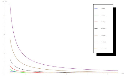 Fig. 6 - How wet you get vs. how fast you run for various wind speeds in mph.
Comparison
I will conclude with a comparison of the two results, to each other and
to the vertical case. First, lets take the appropriate limits.
$$W_{with}=A_f \rho d \left[ (\frac{v_w}{v} - 1)H(v_w -
v)+\delta_{v_w}+\frac{A_t}{A_f} \frac{v_{r,vert}}{v} \right]$$
$$W_{against} = \rho A_f d\left( \left( \frac{A_t}{A_f}\right)
\left(\frac{v_{r,vert}}{v}\right) +\left(\frac{v_w}{v}\right) +
1\right)$$
$$W_{stationary} = \rho t A_f \left(\frac{A_t}{A_f}
v_{r,vert}+v_w\right)$$
$$W_{vert}= \rho d A_f \left(\frac{A_t}{A_f} \frac{v_r}{v} + 1
\right)$$
In the stationary limit, we have to break up the d in our equations into
v t, and that gives
$$\lim_{v \to 0}W_{with}= \lim_{v \to 0} W_{against}=\rho t
A_f \left(\frac{A_t}{A_f} v_{r_vert}+v_w\right)$$
While in the vertical rain limit
$$\lim_{v_w \to 0}W_{with}= \lim_{v_w \to 0} W_{against}
=\rho d A_f \left(\frac{A_t}{A_f} \frac{v_r}{v} + 1 \right)$$
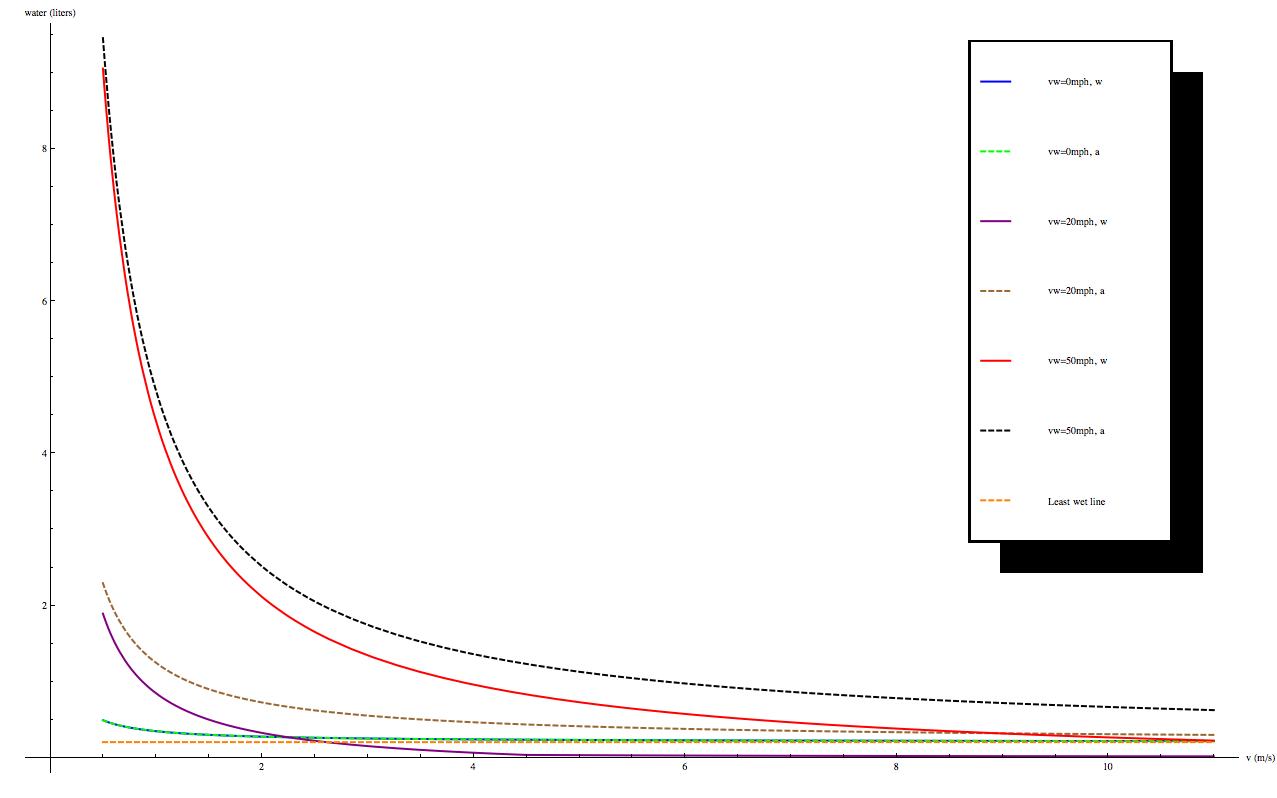
So our limits work. Finally, it's a little hard to tell the difference
between the forward and backwards case, so I've plotted the two lines
together for a few values of v_w. You'll notice that for zero wind
speed they have the same result (which is good, since our limit was the
same), but for the other wind speeds they are remarkably divergent, more
so as you run faster! (again, click to enlarge)
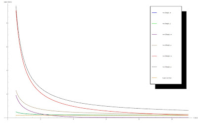 Fig. 7 - Solid lines are running with the rain, dashed lines are running against the rain.
Conclusions
Hopefully this has been an interesting exercise for you. I know it
certainly took me longer to work and write than I initially thought.
While you can't see it in the post, there were a lot of scribblings and
thinking going on before I came to these conclusions. Most of it went
something like: "No, that can't be right, it doesn't have the right
(zero velocity/zero angle) limit!". I think this concludes all of the
running in the rain that I want to do, but if you have more followup
questions, post them below, and I'll do my best to answer. Also, I admit
that my analysis may be a bit rough, so if you have other approaches,
let me know. Finally, note that everything I've found favors running in
the rain, so get yourself some exercise and stay dry!


