This is picture of a watch. (Source: Wikipedia)

A couple of months ago, the Virtuosi Action Team (VAT) assembled for lunch and the discussion quickly and unexpectedly turned to watches. As Nic and Alemi argued over the finer parts of fancy-dancy watch ownership, I looked down at my watch: the lowly Casio F-91W. Though it certainly isn't fancy, it is inexpensive, durable, and could potentially win me an all-expense paid trip to the Caribbean. But how good of a watch is it? To find out, I decided to time it against the official U.S. time for a couple of months. Incidentally, about half-way in I found out that Chad over at Uncertain Principles had done essentially the same thing already. No matter, science is still fun even if you aren't the first person to do it. So here's my "new-to-me" analysis. Alright, so how do we go about quantifying how "good" a watch is? Well, there seem to be two main things we can test. The first of these is accuracy. That is, how close does this watch come to the actual time (according to some time system)? If the official time is 3:00 pm and my watch claims it is 5:00 am, then it is not very accurate. The second measure of "good-ness" is precision or, in watch parlance, stability. This is essentially a measure of the consistency of the watch. If I have a watch that is consistently off by 5 minutes from the official time, then it is not accurate but it is still stable. In essence, a very consistent watch would be just as good as an accurate one, because we can always just subtract off the known offset. To test any of the above measures of how "good" my cheap watch is, we will need to know the actual time. We will adopt the official U.S. time as provided on the NIST website. This time is determined and maintained by a collection of really impressive atomic clocks. One of these is in Colorado and the other is secretly guarded by an ever-vigilant Time Lord (see Figure 1).

Figure 1: Flavor Flav, Keeper of the Time

At 9:00:00 am EST on November 30th, I synchronized my watch with the time displayed on the NIST website. For the next 54 days, I kept track of the difference between my watch an the NIST time. On the 55th day, I forgot to check the time and the experiment promptly ended. The results are plotted below in Figure 2 (and, as with all plots, click through for a larger version).

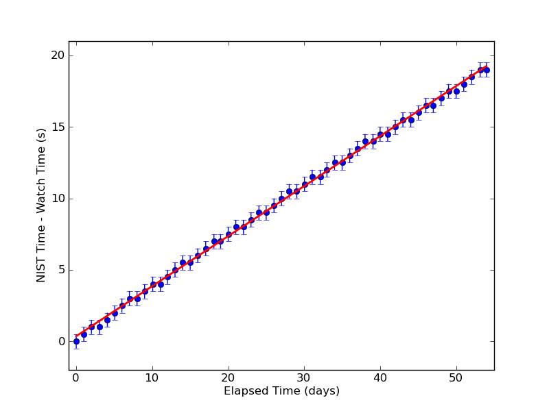Figure 2: Best-fit to time difference

As you can see from Figure 2, the amount of time the watch lost over the timing period appears to be fairly linear. There does appear to be a jagged-ness to the data, though. This is mainly caused by the fact that both the watch and the NIST website only report times to the nearest second. As a result, the finest time resolution I was willing to report was about half a second. Adopting an uncertainty of half a second, I did a least-squares fit of a straight line to the data and found that the watch loses about 0.35 seconds per day. As far as accuracy goes, that's not bad! No matter what, I'll have to set my watch at least twice a year to appease the Daylight Savings Gods. The longest stretch between resetting is about 8 months. If I synchronize my watch with the NIST time to "spring forward" in March, it will only lose about $$ t_{loss} = 8\~\mbox{months} \times 30\frac{\mbox{days}}{\mbox{month}} \times 0.35 \frac{\mbox{sec}}{\mbox{day}} = 84\~\mbox{sec} $$ before I have to re-synchronize to "fall back" in November. Assuming the loss rate is constant, I'll never be more than about a minute and a half off the "actual" time. That's good enough for me. Furthermore, if the watch is consistently losing 0.35 seconds per day and I know how long ago I last synchronized, I can always correct for the offset. In this case, I can always know the official time to within a second (assuming I can add). But is the watch consistent? That's a good question. The simplest means of finding the stability of the watch would be to look at the timing residuals between the data and the model. That is, we will consider how "off" each point is from our constant rate-loss model. A plot of the results is shown below in Figure 3.

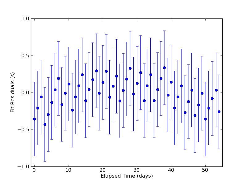Figure 3: Timing residuals

From Figure 3, we see that the data fit the model pretty well. There's a little bit of a wiggle going on there and we see some strong short-term correlations (the latter is an artifact of the fact that I could only get times to the nearest second). To get some sense of the timing stability from the residuals, we can calculate the standard deviation, which will give us a figure for how "off" the data typically are from the model. The standard deviation of the residuals is $$ \sigma_{res} = 0.19\~\mbox{sec}. $$ A good guess at the fractional stability of the watch would then just be the standard deviation divided by the sampling interval, $$ \frac{\sigma_{res}}{T} = 0.19\~\mbox{sec} \times \frac{1}{1\~\mbox{day}} \times \frac{1\~\mbox{day}}{24\times3600\~\mbox{sec}} \approx 2\times10^{-6}.$$ In words, this means that each "tick" of the watch is consistent with the average "tick" value to about 2 parts in a million. That's nice...but isn't there something fancier we could be doing? Well, I have been wanting to learn about Allan variance for some time now, so let's try that. The Allan variance (refs: original paper and a review) can be used to find the fractional frequency stability of an oscillator over a wide range of time scales. Roughly speaking, the Allan variance tells us how averaging our residuals over different chunks of time affects the stability of our data. The square root of the Allan variance, essentially the "Allan standard deviation," is plotted against various averaging times for our data below in Figure 4.

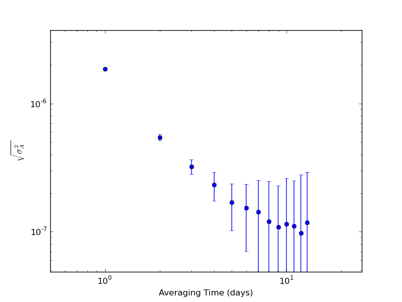Figure 4: Allan variance of our residuals

From Figure 4, we see that as we increase the averaging time from one day to ten days, the Allan deviation decreases. That is, the averaging reduces the amount of variation in the frequency of the data, making it more stable. However, at around 10 days of averaging time it seems as though we hit a floor in how low we can go. Since the error bars get really big here, this may not be a real effect. If it is real, though, this would be indicative of some low-frequency noise in our oscillator. For those who prefer colors, this would be "red" noise. Since the Allan deviation gives the fractional frequency stability of the oscillator, we have that $$\sigma_A = \frac{\delta f}{f} = \frac{\delta(1/t)}{1/t} = \frac{\delta t}{t}. $$ Looking at the plot, we see that with an averaging time of one day, the fractional time stability of the watch is $$\frac{\delta t}{t} \approx 2\times10^{-6}, $$ which corresponds nicely to our previously calculated value. If we average over chunks that are ten days long instead, we get a fractional stability of $$\frac{\delta t}{t} \approx 10^{-7}, $$ which would correspond to a deviation from our model of about 0.008 seconds. Not bad. The initial question that started this whole ordeal was "How good is my watch?" and I think we can safely answer that with "as good as I'll ever need it to be." Hooray for cheap and effective electronics!

Comments