How Cold is the Ground II

Last week (ok, it was a little more than a few days ago...) I used dimensional analysis to figure out how the ground's temperature changes with time. But although dimensional analysis can give us information about the length scales in the problem, it doesn't tell us what the solution looks like. From dimensional analysis, we don't even know what the solution does at large times and distances. (Although we can usually see the asymptotic behavior directly from the equation.) So let's go ahead and solve the the heat equation exactly:

$$ \frac {\partial T}{\partial t} = a \frac {\partial ^2 T}{\partial x^2} \quad (1)$$

Well, what type of solution do we want to this equation? We want the temperature at the Earth's surface $x=0$ to change with the days or the seasons. So let's start out modeling this with a sinusoidal dependence -- we'll look for a solution of the form

$$ T(x,t) = A(x)e^{i wt} $$

for some function $A(x)$, then we can take the real part for our solution. Plugging this into Eq. (1) gives $A^{\prime\prime} = i\omega/a \times A$, or

$$ A(x) = e^{ \pm \sqrt{w/2a } (1+i) x} $$

Since we have a second-order ordinary differential equation for $A$, we have two possible solutions, which are like $\exp(+x)$ or $\exp(-x)$. Which one do we choose?

Well, we want the temperature very far away from the surface of the ground to be constant, so we need the solution that decays with distance, $A\exp(-x)$. Taking the real part of this solution, we find^[1]

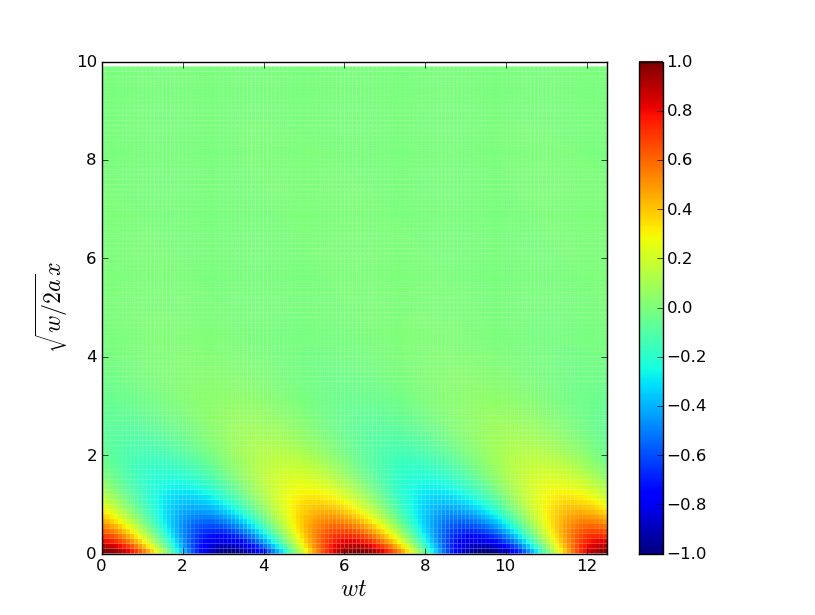
$$ T(x,t) = T_0 \cos (wt + \sqrt{w/2a}\times x ) e^{-\sqrt{w/2a}x} \quad (2) $$

Well, what does this solution say? As we expected from our scaling arguments last week, the distance scale depends on the square root of the time scale -- if we decrease our frequency by 4 (say, looking at changes over a season vs over a month), the ground gets cooler only $2{\times}$ deeper. We also see that the temperature oscillation drops off quite rapidly as we go deeper into the ground, and that there is a "lag" the farther you go into the ground. In particular, we see that at distances deep into the ground, the temperature drops to its average value at the surface. You can see this all in the pretty plot below (generated with Python):

Let's recap. To model the temperature of the ground, we looked for a solution to the heat equation which had a sinusoidally oscillating temperature at $x=0$, and decayed to 0 at large $x$. We found a solution such a solution, and it shows that the temperature decays rapidly as we go far into the ground. At this point, there are two questions that pop into mind:

1) Is the solution that we found unique? Or are there other possible solutions?

2) This is all well and good, but what if our days or seasons aren't perfect sines? Can we find a solution that describes this behavior?

I'll give one (1) VirtuosiPoint to the first commenter who can prove to what extent the above solution is unique^[2]. But how about the second point? Can we solve this for non-sinusoidal time variations? Well, at this point most of the readers are rolling their eyes and shouting "Use a Fourier series and move on." So I will. Briefly, it turns out that (more or less) any periodic function can be written as a sum of sines & cosines. So we can just add a bunch of sines and cosines together and construct our final solution. So just for fun, here is a plot of the temperature of the ground in Ithaca (data from Wikipedia) over a year. (I used a discrete Fourier transform to compute the coefficients.)

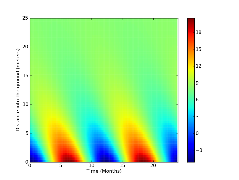
Looks pretty boring, but I swear that all the frequencies are in that plot. It just turns out that the seasons in Ithaca are pretty sinusoidal. So about 20 meters below Ithaca, the temperature is a pretty constant 8 C. While I was postponing writing this, I wondered what the temperature on Mercury's rocks would be. If we dig deep enough, can we find an area with habitable temperatures? Some quick Googlin' shows that the daytime and nighttime temperatures on Mercury are ${\sim}550-700~{\rm K}$ and ${\sim}110~{\rm K}$ at the "equator." While I don't think that Mercury's temperature varies symmetrically, let's assume so for lack of better data.^[3] Then we'd expect that deep into the surface, the temperature would be fairly constant in time, at the average of these two extremes. Plugging in the numbers (assuming $a\approx0.52~{\rm mm}^2 / s$ and using a Mercurial solar day as 176 days), we get

$T=94~{\rm C}$ at 2.75 meters into the surface.

1. ^ More precisely, since the heat equation is linear and real, if $T(x,t)$ is a solution to the equation, then so are $\frac{1}{2}(T+T^{})$ or $\frac{1}{2i}(T-T^{})$.

2. ^ Hint: It's not unique. For instance, here is another solution that satisfies the constraints, with no internal heat sources or sinks (I'll call it the "freshly buried" solution):

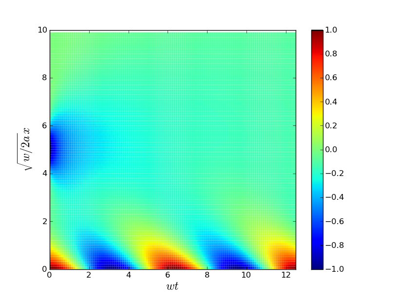
Can you prove that all the other solutions decay to the original solution? Or is there a second or even a spectrum of steady state solutions?

[3] ^ If someone provides me with better data of the time variation of Mercury's surface at some specific latitude, I'll update with a full plot of the temperature as a function of depth and time.